Intro
Discover how to harness the power of XLOOKUP with multiple criteria in Google Sheets. Learn 3 expert-approved methods to search and return data based on multiple conditions, including using arrays, logical operators, and multiple XLOOKUP functions. Unlock advanced data retrieval techniques and streamline your spreadsheet workflow.
Unlocking the Power of XLOOKUP: Mastering Multiple Criteria Searches in Google Sheets
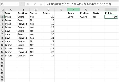
In the world of data analysis, lookup functions are essential tools for extracting specific information from large datasets. Among these functions, XLOOKUP stands out for its flexibility and ease of use. One of the most significant advantages of XLOOKUP is its ability to handle multiple criteria searches, making it an indispensable asset for anyone working with complex data in Google Sheets. In this article, we will delve into the world of XLOOKUP and explore three methods for using this powerful function with multiple criteria.
Understanding XLOOKUP: The Basics

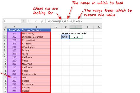
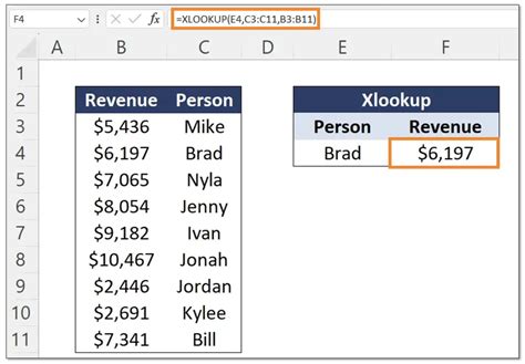
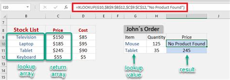
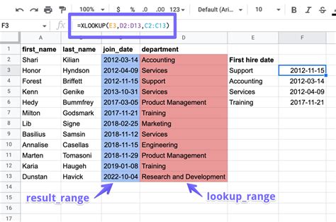
Before we dive into the advanced techniques, it's essential to grasp the fundamentals of XLOOKUP. The function has four primary arguments:
lookup_value: The value you want to search for.lookup_array: The range or array where you want to search for the value.return_array: The range or array from which you want to return a value.[if_not_found]: The value to return if the lookup value is not found.
The basic syntax is: XLOOKUP(lookup_value, lookup_array, return_array, [if_not_found]).
Method 1: Using Multiple Criteria with Separate Columns
One of the most common scenarios where you need to use multiple criteria is when your data is spread across separate columns. Suppose you have a dataset with customer information, including names, addresses, and order numbers, and you want to find the order number for a specific customer based on their name and address.
| Name | Address | Order Number |
|---|---|---|
| John | New York | 123 |
| Jane | Chicago | 456 |
| John | Chicago | 789 |
To achieve this, you can use the following formula:
=XLOOKUP(1, (A2:A10="John") * (B2:B10="Chicago"), C2:C10)
In this example:
A2:A10="John"andB2:B10="Chicago"create arrays of boolean values (TRUE or FALSE) for each row, where the conditions are met.- The
*operator multiplies these arrays, creating a new array with only the rows where both conditions are TRUE. - The
XLOOKUPfunction then searches for the value 1 in this array and returns the corresponding order number from column C.
Method 2: Using Multiple Criteria with a Single Column
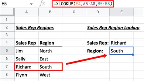
Sometimes, you may have multiple criteria within a single column. For instance, you have a list of product codes with different categories and subcategories, and you want to find the product code that matches a specific category and subcategory.
| Product Code | Category | Subcategory |
|---|---|---|
| ABC | Electronics | Smartphone |
| DEF | Electronics | Laptop |
| GHI | Fashion | Clothing |
To achieve this, you can use the following formula:
=XLOOKUP(1, (A2:A10="Electronics") * (B2:B10="Smartphone"), C2:C10)
In this example, the * operator is used to combine the arrays of boolean values for each row, where the category is "Electronics" and the subcategory is "Smartphone".
Method 3: Using Multiple Criteria with an Array Formula
When working with large datasets, it's not uncommon to have multiple criteria that need to be applied simultaneously. In such cases, using an array formula can be an efficient way to handle multiple criteria searches.
Suppose you have a dataset with sales data, including region, product, and sales amount, and you want to find the total sales amount for a specific region and product.
| Region | Product | Sales Amount |
|---|---|---|
| North | Product A | 100 |
| North | Product B | 200 |
| South | Product A | 300 |
| South | Product B | 400 |
To achieve this, you can use the following formula:
=SUM(FILTER(C2:C10, (A2:A10="North") * (B2:B10="Product A")))
In this example, the FILTER function is used to apply the multiple criteria to the sales amount column, and the SUM function is used to calculate the total sales amount.
Conclusion: Mastering XLOOKUP with Multiple Criteria

In this article, we have explored three methods for using XLOOKUP with multiple criteria in Google Sheets. Whether you're working with separate columns, a single column, or an array formula, these techniques will help you unlock the full potential of XLOOKUP and take your data analysis skills to the next level. Remember to practice these methods and experiment with different scenarios to become proficient in using XLOOKUP with multiple criteria.
Gallery of XLOOKUP Examples
XLOOKUP Examples Gallery




Share Your Thoughts
Have you used XLOOKUP with multiple criteria in your Google Sheets workflows? Share your experiences, tips, and tricks in the comments below!
