
Searching multiple values in Excel can be a daunting task, especially when working with large datasets. However, there are several ways to achieve this, and in this article, we will explore five methods to help you search multiple values in Excel efficiently.
Why Searching Multiple Values is Important

Searching multiple values is essential in various scenarios, such as data analysis, data cleaning, and data visualization. When working with large datasets, it's common to need to find specific values or patterns within the data. Searching multiple values allows you to identify trends, outliers, and correlations, which can inform business decisions or drive further analysis.
Method 1: Using the FILTER Function
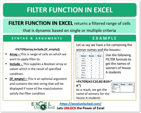
The FILTER function is a new addition to Excel's formula library, introduced in Excel 365. This function allows you to filter a range of cells based on multiple criteria. The syntax for the FILTER function is:
FILTER(range, include, [if_empty])
Where:
- range is the range of cells you want to filter
- include is the criteria you want to apply to the range
- if_empty is an optional argument that specifies what to return if the filtered range is empty
For example, suppose you have a list of sales data with columns for region, product, and sales amount. You can use the FILTER function to find all sales data for a specific region and product:
=FILTER(A2:C10, (A2:A10="North") * (B2:B10="Product A"))
This formula filters the range A2:C10 to include only rows where the region is "North" and the product is "Product A".
Advantages and Limitations of the FILTER Function
The FILTER function is a powerful tool for searching multiple values in Excel. However, it has some limitations:
- It's only available in Excel 365 and later versions
- It can only filter data based on a single range
- It doesn't support wildcard characters or regular expressions
Despite these limitations, the FILTER function is a valuable addition to Excel's formula library, and it can be used to search multiple values in a variety of scenarios.
Method 2: Using the INDEX-MATCH Function Combination
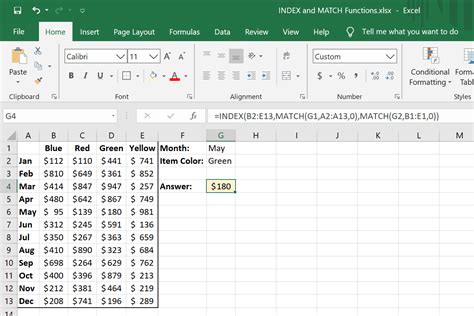
The INDEX-MATCH function combination is a popular method for searching multiple values in Excel. This combination uses the INDEX function to return a value from a range, and the MATCH function to find the relative position of a value within a range.
The syntax for the INDEX-MATCH function combination is:
INDEX(range, MATCH(lookup_value, lookup_array, [match_type]))
Where:
- range is the range of cells you want to search
- lookup_value is the value you want to find
- lookup_array is the range of cells that contains the value you want to find
- match_type is an optional argument that specifies the type of match you want to perform
For example, suppose you have a list of sales data with columns for region, product, and sales amount. You can use the INDEX-MATCH function combination to find all sales data for a specific region and product:
=INDEX(C2:C10, MATCH(1, (A2:A10="North") * (B2:B10="Product A"), 0))
This formula searches the range A2:A10 for the value "North", and the range B2:B10 for the value "Product A". It then returns the corresponding value from the range C2:C10.
Advantages and Limitations of the INDEX-MATCH Function Combination
The INDEX-MATCH function combination is a flexible and powerful method for searching multiple values in Excel. However, it has some limitations:
- It can be slow for large datasets
- It requires careful setup and syntax
- It doesn't support wildcard characters or regular expressions
Despite these limitations, the INDEX-MATCH function combination is a popular method for searching multiple values in Excel, and it can be used in a variety of scenarios.
Method 3: Using the VLOOKUP Function
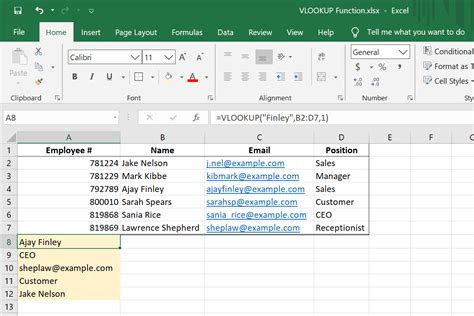
The VLOOKUP function is a popular method for searching multiple values in Excel. This function searches a range of cells for a value, and returns a corresponding value from another range.
The syntax for the VLOOKUP function is:
VLOOKUP(lookup_value, table_array, col_index_num, [range_lookup])
Where:
- lookup_value is the value you want to find
- table_array is the range of cells that contains the value you want to find
- col_index_num is the column number that contains the value you want to return
- range_lookup is an optional argument that specifies the type of match you want to perform
For example, suppose you have a list of sales data with columns for region, product, and sales amount. You can use the VLOOKUP function to find all sales data for a specific region and product:
=VLOOKUP("North", A2:C10, 3, FALSE)
This formula searches the range A2:C10 for the value "North", and returns the corresponding value from the range C2:C10.
Advantages and Limitations of the VLOOKUP Function
The VLOOKUP function is a popular method for searching multiple values in Excel. However, it has some limitations:
- It can be slow for large datasets
- It requires careful setup and syntax
- It doesn't support wildcard characters or regular expressions
Despite these limitations, the VLOOKUP function is a popular method for searching multiple values in Excel, and it can be used in a variety of scenarios.
Method 4: Using the Power Query Editor
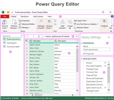
The Power Query Editor is a powerful tool in Excel that allows you to search multiple values in a dataset. This tool uses a graphical interface to filter and transform data, making it easy to search for multiple values.
To use the Power Query Editor, follow these steps:
- Select the range of cells you want to search
- Go to the "Data" tab in the ribbon
- Click on "From Table/Range"
- Click on "Add Column"
- Click on "Filter"
- Enter your search criteria
For example, suppose you have a list of sales data with columns for region, product, and sales amount. You can use the Power Query Editor to find all sales data for a specific region and product:
- Select the range A2:C10
- Go to the "Data" tab in the ribbon
- Click on "From Table/Range"
- Click on "Add Column"
- Click on "Filter"
- Enter the search criteria "Region" = "North" and "Product" = "Product A"
This will filter the data to include only rows where the region is "North" and the product is "Product A".
Advantages and Limitations of the Power Query Editor
The Power Query Editor is a powerful tool for searching multiple values in Excel. However, it has some limitations:
- It can be slow for large datasets
- It requires careful setup and syntax
- It doesn't support wildcard characters or regular expressions
Despite these limitations, the Power Query Editor is a popular method for searching multiple values in Excel, and it can be used in a variety of scenarios.
Method 5: Using the Excel Find and Select Function
The Excel Find and Select function is a simple method for searching multiple values in Excel. This function allows you to search for a value in a range of cells, and then select the corresponding cells.
To use the Find and Select function, follow these steps:
- Select the range of cells you want to search
- Go to the "Home" tab in the ribbon
- Click on "Find and Select"
- Enter your search criteria
For example, suppose you have a list of sales data with columns for region, product, and sales amount. You can use the Find and Select function to find all sales data for a specific region and product:
- Select the range A2:C10
- Go to the "Home" tab in the ribbon
- Click on "Find and Select"
- Enter the search criteria "Region" = "North" and "Product" = "Product A"
This will select the cells that match the search criteria.
Advantages and Limitations of the Excel Find and Select Function
The Excel Find and Select function is a simple method for searching multiple values in Excel. However, it has some limitations:
- It can be slow for large datasets
- It requires careful setup and syntax
- It doesn't support wildcard characters or regular expressions
Despite these limitations, the Excel Find and Select function is a popular method for searching multiple values in Excel, and it can be used in a variety of scenarios.
Excel Search Multiple Values Image Gallery


In conclusion, searching multiple values in Excel can be a challenging task, but there are several methods that can help you achieve this. In this article, we explored five methods for searching multiple values in Excel, including the FILTER function, the INDEX-MATCH function combination, the VLOOKUP function, the Power Query Editor, and the Excel Find and Select function. Each method has its advantages and limitations, and the choice of method depends on the specific scenario and dataset.
We hope this article has been helpful in exploring the different methods for searching multiple values in Excel. If you have any further questions or need more information, please don't hesitate to ask.