Unlocking the Power of Index Match in Google Sheets

Index Match is a powerful combination of functions in Google Sheets that can help you retrieve data from a table or range. While it may seem intimidating at first, mastering Index Match can take your data analysis skills to the next level. In this article, we'll explore five ways to unlock the power of Index Match in Google Sheets.
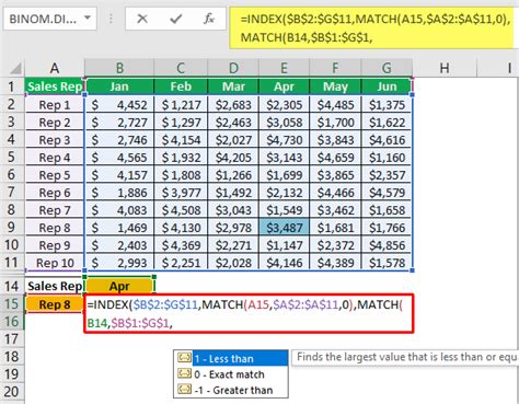
When working with large datasets, finding specific information can be a daunting task. That's where Index Match comes in. By combining the INDEX and MATCH functions, you can create a flexible and dynamic formula that can retrieve data from any column or row.
What is the INDEX Function?
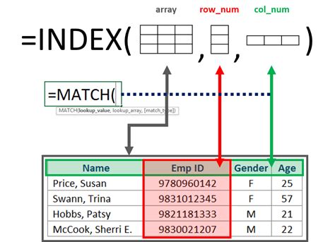
The INDEX function returns a value at a specified position in a range or array. It's like a map that helps you find a specific location in your data. The syntax for the INDEX function is:
=INDEX(range, row, column)
Where range is the array or range of cells you want to search, row is the row number you want to retrieve, and column is the column number you want to retrieve.
What is the MATCH Function?
The MATCH function returns the relative position of a value within a range or array. It's like a search engine that helps you find the location of a specific value. The syntax for the MATCH function is:
=MATCH(lookup_value, range, [match_type])
Where lookup_value is the value you want to search for, range is the array or range of cells you want to search, and match_type is the type of match you want to perform (optional).
5 Ways to Master Index Match in Google Sheets

Now that we've covered the basics of the INDEX and MATCH functions, let's dive into five ways to master Index Match in Google Sheets.
1. Retrieving Data from a Table
One of the most common uses of Index Match is to retrieve data from a table. Let's say you have a table with the following data:
| Name | Age | City |
|---|---|---|
| John | 25 | New York |
| Jane | 30 | London |
| Bob | 35 | Paris |
If you want to retrieve the age of John, you can use the following formula:
=INDEX(B:B, MATCH("John", A:A, 0))
This formula uses the INDEX function to return the value in column B (Age) that corresponds to the value "John" in column A (Name). The MATCH function is used to find the relative position of "John" in column A.
2. Searching for Multiple Criteria
Index Match can also be used to search for multiple criteria. Let's say you have a table with the following data:
| Name | Age | City | Country |
|---|---|---|---|
| John | 25 | New York | USA |
| Jane | 30 | London | UK |
| Bob | 35 | Paris | France |
If you want to retrieve the country of John, who is 25 years old and lives in New York, you can use the following formula:
=INDEX(D:D, MATCH(1, (A:A="John")*(B:B=25)*(C:C="New York"), 0))
This formula uses the INDEX function to return the value in column D (Country) that corresponds to the values "John", 25, and "New York" in columns A, B, and C, respectively. The MATCH function is used to find the relative position of the combination of these values.
3. Retrieving Data from a Pivot Table
Index Match can also be used to retrieve data from a pivot table. Let's say you have a pivot table with the following data:
| City | Total Sales |
|---|---|
| New York | 1000 |
| London | 2000 |
| Paris | 3000 |
If you want to retrieve the total sales for New York, you can use the following formula:
=INDEX(B:B, MATCH("New York", A:A, 0))
This formula uses the INDEX function to return the value in column B (Total Sales) that corresponds to the value "New York" in column A (City). The MATCH function is used to find the relative position of "New York" in column A.
4. Using Index Match with Multiple Sheets
Index Match can also be used to retrieve data from multiple sheets. Let's say you have two sheets, "Sheet1" and "Sheet2", with the following data:
Sheet1
| Name | Age |
|---|---|
| John | 25 |
| Jane | 30 |
| Bob | 35 |
Sheet2
| Name | City |
|---|---|
| John | New York |
| Jane | London |
| Bob | Paris |
If you want to retrieve the city of John, who is 25 years old, you can use the following formula:
=INDEX(Sheet2!B:B, MATCH(1, (Sheet1!A:A="John")*(Sheet1!B:B=25), 0))
This formula uses the INDEX function to return the value in column B (City) of "Sheet2" that corresponds to the values "John" and 25 in columns A and B of "Sheet1", respectively. The MATCH function is used to find the relative position of the combination of these values.
5. Using Index Match with Array Formulas
Index Match can also be used with array formulas to retrieve data from a range or array. Let's say you have a range with the following data:
| Name | Age | City |
|---|---|---|
| John | 25 | New York |
| Jane | 30 | London |
| Bob | 35 | Paris |
If you want to retrieve the names of people who are 25 or older, you can use the following formula:
=INDEX(A:A, N(MATCH(TRUE, B:B>=25, 0)))
This formula uses the INDEX function to return the values in column A (Name) that correspond to the values 25 or older in column B (Age). The MATCH function is used to find the relative position of the values 25 or older in column B.
Gallery of Index Match Formulas in Google Sheets
Index Match Formula Gallery


We hope this article has helped you master the Index Match formula in Google Sheets. With these five examples, you can unlock the power of Index Match and take your data analysis skills to the next level. Whether you're a beginner or an advanced user, Index Match is a powerful tool that can help you retrieve data from tables, pivot tables, and even multiple sheets. Don't forget to experiment with different formulas and examples to get the most out of Index Match.
What's your favorite way to use Index Match in Google Sheets? Share your tips and tricks in the comments below!
