The world of Excel can be overwhelming, especially when it comes to looking up and comparing data. One of the most powerful and commonly used functions in Excel is the VLOOKUP function. In this article, we will delve into the world of VLOOKUP and explore how to compare two columns with ease.
The VLOOKUP function is a game-changer for anyone who works with data. It allows you to search for a value in a table and return a corresponding value from another column. This function is particularly useful when working with large datasets, where manual lookup can be time-consuming and prone to errors.
What is VLOOKUP?

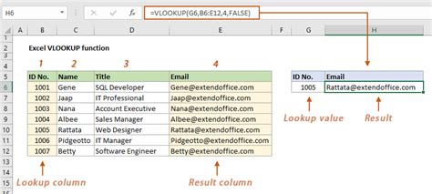
VLOOKUP stands for Vertical Lookup. It is a function that searches for a value in a table and returns a corresponding value from another column. The function takes four arguments: the value to be searched, the table range, the column index, and the range lookup.
How to Use VLOOKUP
Using VLOOKUP is relatively straightforward. Here's a step-by-step guide to get you started:
- Select the cell where you want to display the result.
- Type
=VLOOKUP(to start the function. - Enter the value to be searched, followed by a comma.
- Enter the table range, including the column headers.
- Enter the column index, which is the column number that contains the value you want to return.
- Enter the range lookup, which can be either TRUE or FALSE.
- Close the parentheses and press Enter.
The syntax for VLOOKUP is as follows:
=VLOOKUP(lookup_value, table_array, col_index_num, [range_lookup])
VLOOKUP Examples
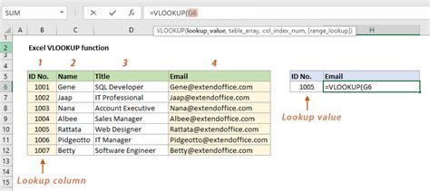
Let's consider a simple example. Suppose we have a table with employee names and their corresponding employee IDs. We want to find the employee ID for a specific employee.
| Employee Name | Employee ID |
|---|---|
| John Smith | 101 |
| Jane Doe | 102 |
| Bob Johnson | 103 |
Using VLOOKUP, we can search for the employee ID for John Smith as follows:
=VLOOKUP("John Smith", A:B, 2, FALSE)
In this example, the lookup value is "John Smith", the table range is A:B, the column index is 2 (since the employee ID is in the second column), and the range lookup is FALSE (since we want an exact match).
Comparing Two Columns with VLOOKUP
Now that we've covered the basics of VLOOKUP, let's move on to comparing two columns. Suppose we have two tables, each with a column of employee names. We want to find the employees who are present in both tables.
| Employee Name | Employee Name | |
|---|---|---|
| John Smith | John Smith | |
| Jane Doe | Bob Johnson | |
| Bob Johnson | Alice Brown |
Using VLOOKUP, we can compare the two columns as follows:
=VLOOKUP(A2, E:F, 1, FALSE)
In this example, the lookup value is the employee name in cell A2, the table range is E:F, the column index is 1 (since we want to return the employee name), and the range lookup is FALSE (since we want an exact match).
We can then use the IF function to check if the result is not an error, indicating that the employee is present in both tables.
=IF(ISERROR(VLOOKUP(A2, E:F, 1, FALSE)), "Not Found", "Found")
VLOOKUP vs INDEX/MATCH
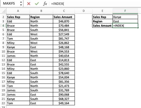
While VLOOKUP is a powerful function, it has its limitations. One of the main limitations is that it can only search for values in the first column of the table range. If you need to search for values in other columns, you'll need to use the INDEX/MATCH function combination.
The INDEX/MATCH function combination is more flexible and powerful than VLOOKUP. It allows you to search for values in any column of the table range and return a corresponding value from another column.
Here's an example of how to use the INDEX/MATCH function combination:
=INDEX(C:C, MATCH(A2, B:B, 0))
In this example, the INDEX function returns the value in column C, based on the relative position of the value in column B.
Benefits of Using VLOOKUP
- Easy to use: VLOOKUP is a straightforward function to use, even for those who are new to Excel.
- Fast and efficient: VLOOKUP can search large datasets quickly and efficiently.
- Flexible: VLOOKUP can be used to search for values in any column of the table range.
- Easy to read: VLOOKUP formulas are easy to read and understand, making it easier to maintain and update your spreadsheets.
Common VLOOKUP Errors
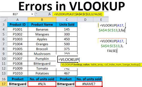
While VLOOKUP is a powerful function, it's not without its errors. Here are some common VLOOKUP errors to watch out for:
- #N/A error: This error occurs when the lookup value is not found in the table range.
- #REF! error: This error occurs when the column index is incorrect.
- #VALUE! error: This error occurs when the lookup value is not a number.
To avoid these errors, make sure to double-check your VLOOKUP formulas and ensure that the lookup value is correct and the column index is accurate.
Best Practices for Using VLOOKUP
- Use absolute references: Use absolute references for the table range and column index to avoid errors when copying and pasting formulas.
- Use named ranges: Use named ranges to make your VLOOKUP formulas more readable and easier to maintain.
- Avoid using VLOOKUP with large datasets: VLOOKUP can slow down your spreadsheet if used with large datasets. Consider using the INDEX/MATCH function combination instead.
Conclusion
In conclusion, VLOOKUP is a powerful function that can help you compare two columns with ease. While it has its limitations, it's a great tool to have in your Excel toolkit. By following the best practices outlined in this article, you can avoid common VLOOKUP errors and use the function to its full potential.
What's your favorite way to use VLOOKUP? Share your tips and tricks in the comments below!
VLOOKUP Image Gallery

