Intro
Master Excels VLOOKUP with Concatenate function and streamline your data analysis. This step-by-step guide teaches you how to combine VLOOKUP with Concatenate to search and retrieve data from complex tables, improving your lookup and reference skills. Learn how to efficiently merge data, create dynamic lookups, and automate tasks using Excel formulas and functions.
Using Excel Vlookup with Concatenate can be a powerful tool to retrieve data from a table by looking up a value in a different column. The Vlookup function in Excel is used to search for a value in the first column of a table and return a value in the same row from another column. However, there are situations where you need to look up a value based on multiple criteria, and that's where the Concatenate function comes in. In this article, we will explore how to use Excel Vlookup with Concatenate to solve complex lookup problems.
Understanding the Vlookup Function

The Vlookup function in Excel is used to search for a value in the first column of a table and return a value in the same row from another column. The syntax for the Vlookup function is as follows:
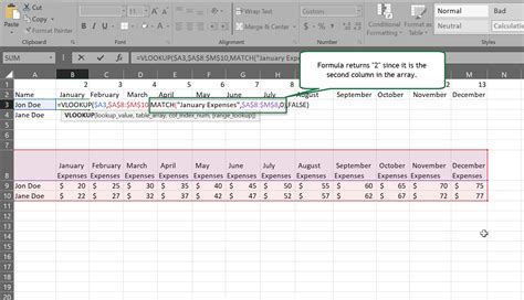
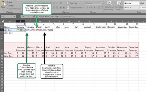
VLOOKUP(lookup_value, table_array, col_index_num, [range_lookup])
- lookup_value is the value you want to look up.
- table_array is the range of cells that contains the data you want to search.
- col_index_num is the column number that contains the value you want to return.
- [range_lookup] is a logical value that specifies whether you want an exact match or an approximate match.
Understanding the Concatenate Function
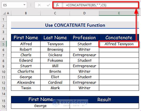
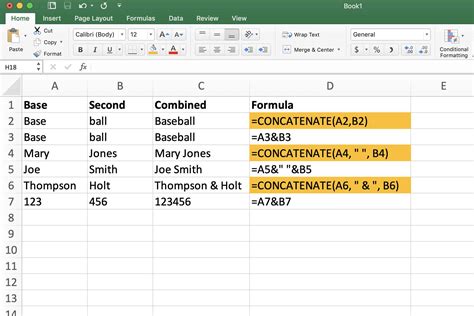
The Concatenate function in Excel is used to join two or more text strings into a single text string. The syntax for the Concatenate function is as follows:
CONCATENATE(text1, [text2],...)
- text1 is the first text string you want to join.
- [text2] is the second text string you want to join, and so on.
Using Excel Vlookup with Concatenate
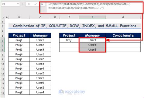
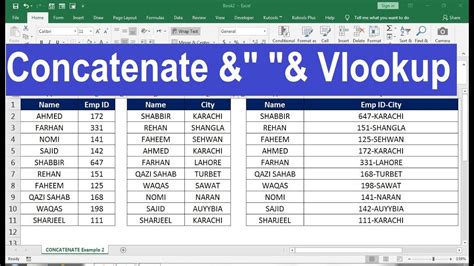
To use Excel Vlookup with Concatenate, you need to concatenate the multiple criteria you want to look up into a single text string, and then use the Vlookup function to search for that text string in the first column of the table.
Here's an example:
Suppose you have a table with the following columns:
| Employee ID | First Name | Last Name | Department |
|---|---|---|---|
| 101 | John | Smith | Sales |
| 102 | Jane | Doe | Marketing |
| 103 | Bob | Johnson | Sales |
You want to look up the department of an employee based on their first name and last name. You can use the Concatenate function to join the first name and last name into a single text string, and then use the Vlookup function to search for that text string in the first column of the table.
The formula would be:
=VLOOKUP(CONCATENATE(A2, " ", B2), table_array, 4, FALSE)
- A2 is the cell that contains the first name.
- B2 is the cell that contains the last name.
- table_array is the range of cells that contains the data you want to search.
- 4 is the column number that contains the department.
- FALSE means you want an exact match.
Example 2: Using Excel Vlookup with Concatenate to Search for Multiple Criteria
Suppose you have a table with the following columns:
| Order ID | Customer ID | Order Date | Total |
|---|---|---|---|
| 1001 | 101 | 2022-01-01 | 100 |
| 1002 | 102 | 2022-01-02 | 200 |
| 1003 | 103 | 2022-01-03 | 300 |
You want to look up the total of an order based on the customer ID and order date. You can use the Concatenate function to join the customer ID and order date into a single text string, and then use the Vlookup function to search for that text string in the first column of the table.
The formula would be:
=VLOOKUP(CONCATENATE(A2, " ", B2), table_array, 4, FALSE)
- A2 is the cell that contains the customer ID.
- B2 is the cell that contains the order date.
- table_array is the range of cells that contains the data you want to search.
- 4 is the column number that contains the total.
- FALSE means you want an exact match.
Tips and Tricks for Using Excel Vlookup with Concatenate
- Make sure to use the Concatenate function to join the multiple criteria into a single text string.
- Use the Vlookup function to search for the concatenated text string in the first column of the table.
- Use the FALSE argument to specify an exact match.
- Use the column number to specify the column that contains the value you want to return.
- Use the table_array argument to specify the range of cells that contains the data you want to search.
Common Errors to Avoid When Using Excel Vlookup with Concatenate
- Make sure to use the correct syntax for the Vlookup and Concatenate functions.
- Make sure to specify the correct column number and table array.
- Make sure to use the FALSE argument to specify an exact match.
- Avoid using the Vlookup function with Concatenate on large datasets, as it can be slow and inefficient.
Excel Vlookup with Concatenate Image Gallery



Conclusion
Using Excel Vlookup with Concatenate can be a powerful tool to retrieve data from a table by looking up multiple criteria. By following the steps outlined in this article, you can use the Concatenate function to join multiple criteria into a single text string, and then use the Vlookup function to search for that text string in the first column of the table. Remember to use the correct syntax, specify the correct column number and table array, and avoid common errors. With practice and patience, you can master the use of Excel Vlookup with Concatenate and improve your data analysis skills.
We hope this article has been helpful in explaining how to use Excel Vlookup with Concatenate. If you have any questions or need further assistance, please don't hesitate to ask. Share your thoughts and experiences in the comments section below, and don't forget to share this article with your friends and colleagues who may benefit from it.
