Create A Pie In A Pie Chart In Excel Easily

Creating a pie in a pie chart, also known as a nested pie chart or a pie chart within a pie chart, can be a visually appealing way to display data in Excel. This type of chart is useful when you want to show the relationship between two sets of data, where one set is a subset of the other.

Understanding the Basics of a Pie in a Pie Chart

Before we dive into the steps to create a pie in a pie chart in Excel, let's understand the basics of this type of chart. A pie in a pie chart consists of two concentric circles, where the larger circle represents the main data series and the smaller circle represents the subset of data.

Advantages of a Pie in a Pie Chart

1. Visual appeal: A pie in a pie chart is a visually appealing way to display data, making it easy to understand and analyze.
2. Relationship between data: This type of chart helps to show the relationship between two sets of data, where one set is a subset of the other.
3. Easy to create: With the steps outlined below, creating a pie in a pie chart in Excel is easy and straightforward.

Step-by-Step Guide to Creating a Pie in a Pie Chart in Excel

Creating a pie in a pie chart in Excel is a straightforward process. Here are the steps:

Step 1: Prepare Your Data

Before creating the chart, you need to prepare your data. Make sure you have two sets of data, where one set is a subset of the other.

• Data Set 1: This is the main data series that will be represented by the larger circle.
• Data Set 2: This is the subset of data that will be represented by the smaller circle.

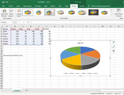
Step 2: Create a New Chart

To create a new chart in Excel, follow these steps:

1. Select the data range that you want to use for the chart.
2. Go to the "Insert" tab in the ribbon.
3. Click on the "Pie Chart" button in the "Charts" group.
4. Select "Pie in Pie Chart" from the drop-down menu.

Step 3: Customize the Chart

Once you have created the chart, you can customize it to suit your needs. Here are a few things you can do:

• Change the chart title: Click on the chart title and type in a new title.
• Change the data series: Right-click on the chart and select "Select Data" to change the data series.
• Change the colors: Right-click on the chart and select "Format Data Series" to change the colors.

Step 4: Add the Second Pie Chart

To add the second pie chart, follow these steps:

1. Right-click on the chart and select "Select Data".
2. Click on the "Add" button to add a new data series.
3. Select the data range for the second pie chart.
4. Click "OK" to add the second pie chart.

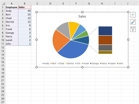
Step 5: Format the Second Pie Chart

Once you have added the second pie chart, you can format it to suit your needs. Here are a few things you can do:

• Change the size: Right-click on the second pie chart and select "Format Data Series" to change the size.
• Change the colors: Right-click on the second pie chart and select "Format Data Series" to change the colors.

Tips and Tricks for Creating a Pie in a Pie Chart in Excel

Here are a few tips and tricks to help you create a pie in a pie chart in Excel:

• Use a consistent color scheme: Use a consistent color scheme to make the chart easy to read and understand.
• Use a clear and concise title: Use a clear and concise title to explain the chart.
• Use data labels: Use data labels to make the chart easy to read and understand.

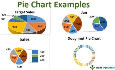
Gallery of Pie in a Pie Chart Examples

Pie in a Pie Chart Examples

By following these steps and tips, you can create a visually appealing pie in a pie chart in Excel that effectively communicates your data insights.

If you have any questions or need further clarification, please don't hesitate to comment below.