
Creating a risk heat map in Excel is a valuable skill for professionals across various industries, as it enables them to visualize and prioritize potential risks in a clear and concise manner. A risk heat map is a graphical representation of the likelihood and impact of different risks, allowing users to quickly identify areas that require attention. In this article, we will explore five ways to create a risk heat map in Excel, providing step-by-step instructions and practical examples to help you get started.
Understanding Risk Heat Maps

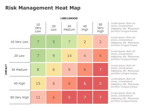
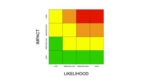
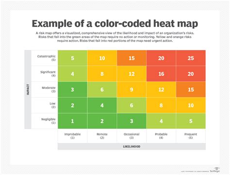
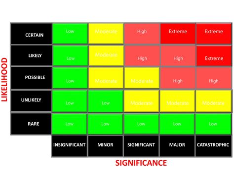
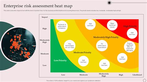
Before we dive into the different methods for creating risk heat maps in Excel, it's essential to understand the basics. A risk heat map typically consists of a matrix with two axes: likelihood (or probability) on one axis and impact (or severity) on the other. Each risk is plotted on the matrix based on its likelihood and impact scores, resulting in a visual representation of the risk landscape.
Benefits of Using Risk Heat Maps
Risk heat maps offer several benefits, including:
- Clear visualization of potential risks
- Easy identification of high-priority risks
- Ability to prioritize risk mitigation efforts
- Enhanced communication and collaboration among stakeholders
- Simplified risk assessment and monitoring
Method 1: Using Conditional Formatting
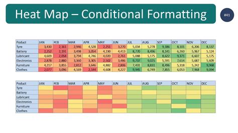
One of the simplest ways to create a risk heat map in Excel is by using conditional formatting. This method involves creating a table with likelihood and impact scores, and then applying conditional formatting rules to highlight cells based on their values.
To create a risk heat map using conditional formatting, follow these steps:
- Set up a table with likelihood and impact scores for each risk
- Select the cells containing the scores
- Go to the "Home" tab in the Excel ribbon
- Click on "Conditional Formatting" and select "New Rule"
- Choose "Use a formula to determine which cells to format"
- Enter a formula to determine the formatting based on the scores (e.g., =IF(A2*B2>5,"High Risk","Low Risk"))
- Choose a format for the cells (e.g., fill color, font color)
- Repeat steps 4-7 for each risk level (e.g., high, medium, low)
Example:
Suppose we have a table with likelihood and impact scores for five risks, and we want to create a risk heat map using conditional formatting.
| Risk | Likelihood | Impact |
|---|---|---|
| Risk 1 | 3 | 4 |
| Risk 2 | 2 | 3 |
| Risk 3 | 4 | 2 |
| Risk 4 | 1 | 1 |
| Risk 5 | 5 | 5 |
Using conditional formatting, we can create a risk heat map that highlights cells based on their likelihood and impact scores.
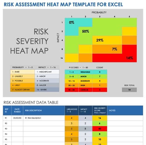
Method 2: Using a Heat Map Template
Another way to create a risk heat map in Excel is by using a pre-designed heat map template. This method involves downloading a heat map template from the internet or creating one from scratch, and then customizing it to fit your specific needs.
To create a risk heat map using a heat map template, follow these steps:
- Download a heat map template from the internet or create one from scratch
- Customize the template to fit your specific needs (e.g., add columns for likelihood and impact scores)
- Enter your risk data into the template
- Use formulas and formatting to create a risk heat map
Example:
Suppose we download a heat map template from the internet and customize it to fit our specific needs.
| Risk | Likelihood | Impact |
|---|---|---|
| Risk 1 | 3 | 4 |
| Risk 2 | 2 | 3 |
| Risk 3 | 4 | 2 |
| Risk 4 | 1 | 1 |
| Risk 5 | 5 | 5 |
Using the heat map template, we can create a risk heat map that visualizes the likelihood and impact scores for each risk.
Method 3: Using a Pivot Table
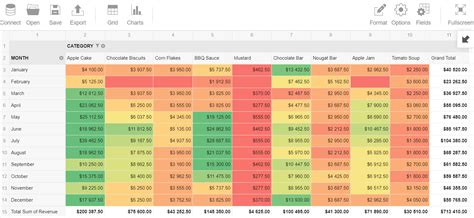
A pivot table is a powerful tool in Excel that can be used to create a risk heat map. This method involves creating a pivot table with likelihood and impact scores, and then using formatting and filtering to create a risk heat map.
To create a risk heat map using a pivot table, follow these steps:
- Set up a table with likelihood and impact scores for each risk
- Create a pivot table based on the table data
- Drag the likelihood and impact scores to the pivot table
- Use formatting and filtering to create a risk heat map
Example:
Suppose we create a pivot table based on the following data:
| Risk | Likelihood | Impact |
|---|---|---|
| Risk 1 | 3 | 4 |
| Risk 2 | 2 | 3 |
| Risk 3 | 4 | 2 |
| Risk 4 | 1 | 1 |
| Risk 5 | 5 | 5 |
Using the pivot table, we can create a risk heat map that visualizes the likelihood and impact scores for each risk.
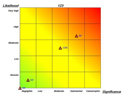
Method 4: Using a Chart

A chart is another way to create a risk heat map in Excel. This method involves creating a chart with likelihood and impact scores, and then using formatting and filtering to create a risk heat map.
To create a risk heat map using a chart, follow these steps:
- Set up a table with likelihood and impact scores for each risk
- Create a chart based on the table data
- Use formatting and filtering to create a risk heat map
Example:
Suppose we create a chart based on the following data:
| Risk | Likelihood | Impact |
|---|---|---|
| Risk 1 | 3 | 4 |
| Risk 2 | 2 | 3 |
| Risk 3 | 4 | 2 |
| Risk 4 | 1 | 1 |
| Risk 5 | 5 | 5 |
Using the chart, we can create a risk heat map that visualizes the likelihood and impact scores for each risk.
Method 5: Using a Third-Party Add-in
A third-party add-in is a software program that can be installed in Excel to create a risk heat map. This method involves installing a third-party add-in, and then using it to create a risk heat map.
To create a risk heat map using a third-party add-in, follow these steps:
- Install a third-party add-in for creating risk heat maps
- Set up a table with likelihood and impact scores for each risk
- Use the add-in to create a risk heat map
Example:
Suppose we install a third-party add-in for creating risk heat maps, and then use it to create a risk heat map based on the following data:
| Risk | Likelihood | Impact |
|---|---|---|
| Risk 1 | 3 | 4 |
| Risk 2 | 2 | 3 |
| Risk 3 | 4 | 2 |
| Risk 4 | 1 | 1 |
| Risk 5 | 5 | 5 |
Using the third-party add-in, we can create a risk heat map that visualizes the likelihood and impact scores for each risk.
Conclusion
Creating a risk heat map in Excel is a valuable skill that can help professionals across various industries to visualize and prioritize potential risks. In this article, we explored five ways to create a risk heat map in Excel, including using conditional formatting, a heat map template, a pivot table, a chart, and a third-party add-in. By following the steps and examples provided, you can create a risk heat map that helps you to identify and prioritize risks in a clear and concise manner.
Risk Heat Map Image Gallery


I hope this article has provided you with valuable insights and practical examples on how to create a risk heat map in Excel. By following the methods and steps outlined in this article, you can create a risk heat map that helps you to identify and prioritize risks in a clear and concise manner.