
Are you tired of struggling with complex formulas in Google Sheets to sum values based on multiple criteria? Look no further! In this article, we'll break down the process of using SUMIF with multiple criteria in Google Sheets, making it easy for you to analyze and summarize your data.
SUMIF is a powerful function in Google Sheets that allows you to sum values based on a single criterion. However, when you need to sum values based on multiple criteria, things can get a bit tricky. But don't worry, we've got you covered!
Understanding SUMIF with Multiple Criteria
Before we dive into the details, let's quickly review how SUMIF works with a single criterion. The syntax for SUMIF is:
SUMIF(range, criterion, [sum_range])
- Range: The range of cells that you want to apply the criterion to.
- Criterion: The condition that you want to apply to the range.
- Sum_range: The range of cells that you want to sum.
When you need to sum values based on multiple criteria, you can use the following syntax:
SUMIFS(sum_range, range1, criterion1, [range2], [criterion2],...)
- Sum_range: The range of cells that you want to sum.
- Range1, range2,...: The ranges of cells that you want to apply the criteria to.
- Criterion1, criterion2,...: The conditions that you want to apply to the ranges.
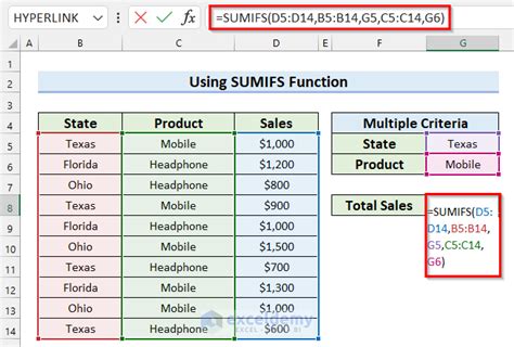
Example: Summing Sales Based on Region and Product
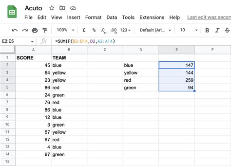
Suppose you have a dataset that contains sales data for different regions and products. You want to sum the sales for the "North" region and "Product A". Here's how you can use SUMIFS to achieve this:
=SUMIFS(D:D, A:A, "North", B:B, "Product A")
In this example:
- D:D is the sum_range (the range of cells that contains the sales values).
- A:A is the range1 (the range of cells that contains the region values).
- "North" is the criterion1 (the condition that you want to apply to the region values).
- B:B is the range2 (the range of cells that contains the product values).
- "Product A" is the criterion2 (the condition that you want to apply to the product values).
Tips and Tricks for Using SUMIFS
Here are some tips and tricks to help you get the most out of SUMIFS:
- Use absolute references: When using SUMIFS, it's a good idea to use absolute references for the ranges and criteria. This will ensure that the formula works correctly even when you insert or delete rows or columns.
- Use named ranges: Named ranges can make your formulas more readable and easier to maintain. You can define named ranges for the ranges and criteria, and then use those named ranges in the SUMIFS formula.
- Use wildcards: Wildcards can be useful when you need to sum values based on partial matches. For example, if you want to sum sales for all products that start with "A", you can use the wildcard "A" in the criterion.
Common Errors to Avoid
Here are some common errors to avoid when using SUMIFS:
- Incorrect range references: Make sure that the range references are correct and absolute.
- Incorrect criteria: Make sure that the criteria are correct and formatted correctly.
- Missing or extra commas: Make sure that there are no missing or extra commas in the formula.
Alternatives to SUMIFS
While SUMIFS is a powerful function, there are alternative functions that you can use to achieve similar results. Here are a few alternatives:
- SUMPRODUCT: SUMPRODUCT is a function that allows you to sum values based on multiple criteria. It's similar to SUMIFS, but it's more flexible and can handle multiple criteria more easily.
- FILTER: FILTER is a function that allows you to filter data based on multiple criteria. You can use it to sum values based on multiple criteria by using the FILTER function to filter the data, and then using the SUM function to sum the filtered data.
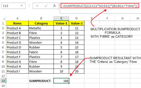
Example: Using SUMPRODUCT to Sum Sales
Suppose you have a dataset that contains sales data for different regions and products. You want to sum the sales for the "North" region and "Product A". Here's how you can use SUMPRODUCT to achieve this:
=SUMPRODUCT((A:A="North")(B:B="Product A")(D:D))
In this example:
- A:A is the range of cells that contains the region values.
- "North" is the criterion1 (the condition that you want to apply to the region values).
- B:B is the range of cells that contains the product values.
- "Product A" is the criterion2 (the condition that you want to apply to the product values).
- D:D is the sum_range (the range of cells that contains the sales values).
Conclusion
In conclusion, SUMIFS is a powerful function in Google Sheets that allows you to sum values based on multiple criteria. By following the tips and tricks outlined in this article, you can use SUMIFS to analyze and summarize your data with ease. Remember to use absolute references, named ranges, and wildcards to make your formulas more readable and maintainable. And don't forget to check out the alternatives to SUMIFS, such as SUMPRODUCT and FILTER, which can also be used to achieve similar results.
Google Sheets Functions Image Gallery


We hope this article has helped you to understand how to use SUMIFS in Google Sheets. If you have any questions or need further clarification, please don't hesitate to ask.