Excel Sumif For Filtered Rows: Simplified Formula And Examples

Excel is an incredibly powerful tool for data analysis, and one of its most useful features is the ability to sum data based on specific criteria using the SUMIF function. However, when dealing with filtered rows, things can get a bit more complicated. In this article, we'll explore how to use the SUMIF function for filtered rows, provide a simplified formula, and walk through some practical examples.

Understanding the SUMIF Function

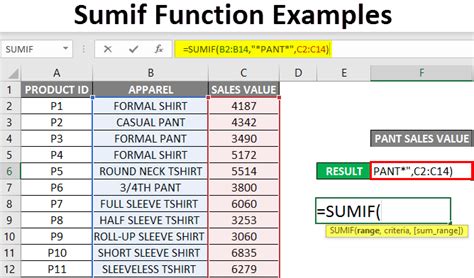
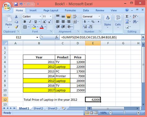
The SUMIF function is used to sum a range of cells based on a specific criteria. The syntax for the SUMIF function is:

SUMIF(range, criteria, [sum_range])

Where:

• range is the range of cells that you want to apply the criteria to
• criteria is the condition that you want to apply to the range
• [sum_range] is the range of cells that you want to sum (optional)

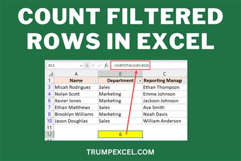
Filtered Rows and the SUBTOTAL Function

When working with filtered rows, the SUMIF function can be a bit tricky to use. This is because the SUMIF function doesn't automatically exclude filtered rows from the calculation. To overcome this limitation, we can use the SUBTOTAL function in combination with the SUMIF function.

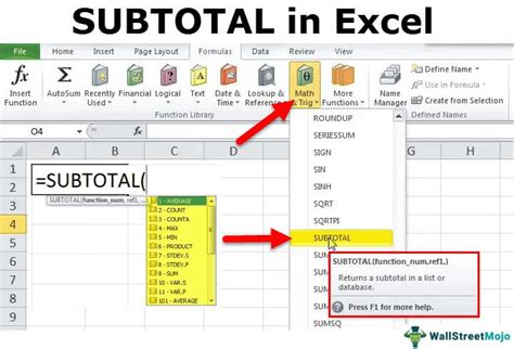
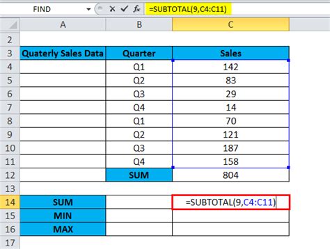
The SUBTOTAL function is used to sum a range of cells, but it automatically excludes filtered rows from the calculation. The syntax for the SUBTOTAL function is:

SUBTOTAL(function_num, ref1, [ref2],...)

Where:

• function_num is a number that specifies the function to use (109 for SUM)
• ref1 is the range of cells that you want to sum
• [ref2] is an optional range of cells to sum

Simplified Formula for SUMIF with Filtered Rows

Here's a simplified formula that combines the SUMIF and SUBTOTAL functions to sum filtered rows:

=SUBTOTAL(109, SUMIF(range, criteria, sum_range))

This formula uses the SUBTOTAL function to sum the results of the SUMIF function, which automatically excludes filtered rows from the calculation.

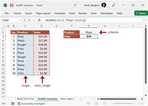
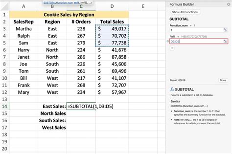
Example 1: Summing Sales by Region

Let's say we have a list of sales data by region, and we want to sum the sales for each region using the SUMIF function. We can use the following formula:

=SUMIF(A2:A10, "North", B2:B10)

Where:

• A2:A10 is the range of cells containing the region names
• "North" is the criteria that we want to apply
• B2:B10 is the range of cells containing the sales data

If we want to sum the sales for the North region, but only for the rows that are not filtered out, we can use the following formula:

=SUBTOTAL(109, SUMIF(A2:A10, "North", B2:B10))

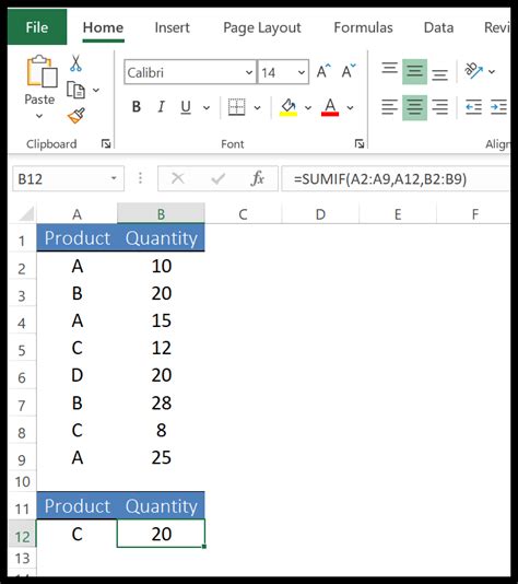
Example 2: Summing Expenses by Category

Let's say we have a list of expense data by category, and we want to sum the expenses for each category using the SUMIF function. We can use the following formula:

=SUMIF(A2:A10, "Travel", B2:B10)

Where:

• A2:A10 is the range of cells containing the category names
• "Travel" is the criteria that we want to apply
• B2:B10 is the range of cells containing the expense data

If we want to sum the expenses for the Travel category, but only for the rows that are not filtered out, we can use the following formula:

=SUBTOTAL(109, SUMIF(A2:A10, "Travel", B2:B10))

Excel SUMIF Function Image Gallery

Conclusion

In this article, we've explored how to use the SUMIF function for filtered rows in Excel. We've provided a simplified formula that combines the SUMIF and SUBTOTAL functions to sum filtered rows, and walked through some practical examples. We hope this article has been helpful in simplifying your Excel workflows. If you have any questions or comments, please feel free to share them below!