5 Ways To Master Vlookup With Two Excel Workbooks

Are you tired of switching between multiple Excel workbooks to find and match data? Do you struggle with using VLOOKUP to extract information from one workbook to another? You're not alone. Many Excel users face this challenge, but with the right techniques, you can master VLOOKUP and boost your productivity.

In this article, we'll explore five ways to use VLOOKUP with two Excel workbooks. You'll learn how to set up your workbooks, create formulas, and troubleshoot common issues. Whether you're a beginner or an advanced user, these methods will help you to efficiently retrieve data from one workbook to another.

Understanding VLOOKUP

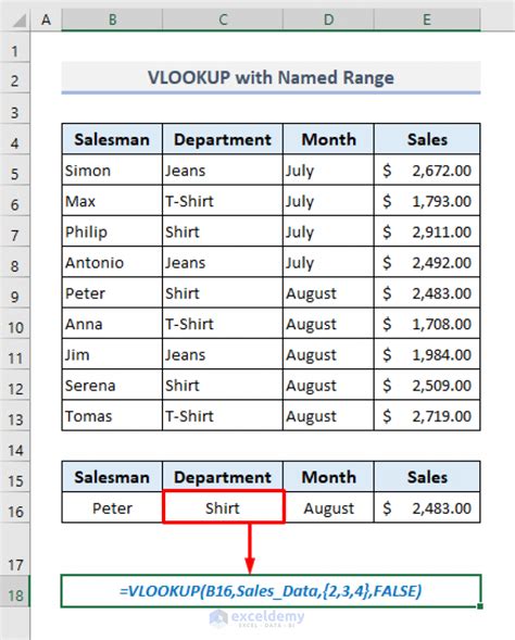
Before we dive into the five methods, let's quickly review how VLOOKUP works. VLOOKUP is a powerful Excel function that allows you to search for a value in a table and return a corresponding value from another column. The syntax is as follows:

VLOOKUP(lookup value, table array, col index num, [range lookup])

• Lookup value: The value you want to search for.
• Table array: The range of cells that contains the data you want to search.
• Col index num: The column number that contains the value you want to return.
• [Range lookup]: Optional, specifies whether you want an exact or approximate match.

Method 1: Using VLOOKUP with Two Workbooks

In this method, we'll use VLOOKUP to retrieve data from one workbook to another using a simple formula.

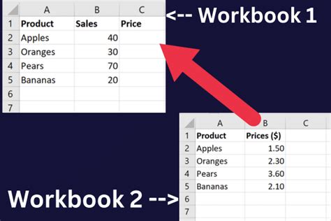
Assuming you have two workbooks: "Workbook1" and "Workbook2". In Workbook1, you have a table with employee IDs and names, and in Workbook2, you have a table with employee IDs and salaries.

To use VLOOKUP, follow these steps:

1. Open both workbooks and select the cell where you want to display the result in Workbook1.
2. Type the VLOOKUP formula: =VLOOKUP(A2, [Workbook2.xlsx]Sheet1!$A$2:$B$10, 2, FALSE)
3. Press Enter to execute the formula.

In this formula:

• A2 is the lookup value (employee ID).
• [Workbook2.xlsx]Sheet1!$A$2:$B$10 is the table array (employee IDs and salaries in Workbook2).
• 2 is the column index number (salaries).
• FALSE specifies an exact match.

Method 2: Using VLOOKUP with Multiple Criteria

In this method, we'll use VLOOKUP with multiple criteria to retrieve data from one workbook to another.

Assuming you have two workbooks: "Workbook1" and "Workbook2". In Workbook1, you have a table with employee IDs, names, and departments, and in Workbook2, you have a table with employee IDs, salaries, and departments.

To use VLOOKUP with multiple criteria, follow these steps:

1. Open both workbooks and select the cell where you want to display the result in Workbook1.
2. Type the VLOOKUP formula: =VLOOKUP(A2&B2, [Workbook2.xlsx]Sheet1!$A$2:$C$10, 3, FALSE)
3. Press Enter to execute the formula.

In this formula:

• A2&B2 is the lookup value (employee ID and department).
• [Workbook2.xlsx]Sheet1!$A$2:$C$10 is the table array (employee IDs, salaries, and departments in Workbook2).
• 3 is the column index number (salaries).
• FALSE specifies an exact match.

Method 3: Using VLOOKUP with Dynamic Ranges

In this method, we'll use VLOOKUP with dynamic ranges to retrieve data from one workbook to another.

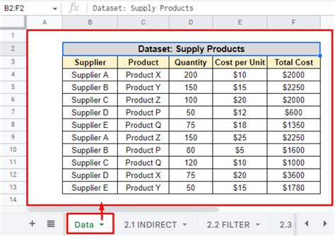
Assuming you have two workbooks: "Workbook1" and "Workbook2". In Workbook1, you have a table with employee IDs and names, and in Workbook2, you have a table with employee IDs and salaries.

To use VLOOKUP with dynamic ranges, follow these steps:

1. Open both workbooks and select the cell where you want to display the result in Workbook1.
2. Type the VLOOKUP formula: =VLOOKUP(A2, OFFSET([Workbook2.xlsx]Sheet1!$A$1, 0, 0, COUNTA([Workbook2.xlsx]Sheet1!$A:$A), 2), 2, FALSE)
3. Press Enter to execute the formula.

In this formula:

• A2 is the lookup value (employee ID).
• OFFSET([Workbook2.xlsx]Sheet1!$A$1, 0, 0, COUNTA([Workbook2.xlsx]Sheet1!$A:$A), 2) is the dynamic range (employee IDs and salaries in Workbook2).
• 2 is the column index number (salaries).
• FALSE specifies an exact match.

Method 4: Using VLOOKUP with Multiple Workbooks

In this method, we'll use VLOOKUP to retrieve data from multiple workbooks.

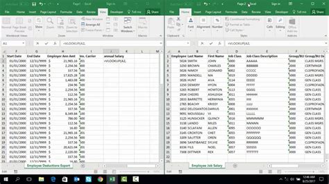
Assuming you have three workbooks: "Workbook1", "Workbook2", and "Workbook3". In Workbook1, you have a table with employee IDs and names, in Workbook2, you have a table with employee IDs and salaries, and in Workbook3, you have a table with employee IDs and departments.

To use VLOOKUP with multiple workbooks, follow these steps:

1. Open all three workbooks and select the cell where you want to display the result in Workbook1.
2. Type the VLOOKUP formula: =VLOOKUP(A2, [Workbook2.xlsx]Sheet1!$A$2:$B$10, 2, FALSE)
3. Press Enter to execute the formula.
4. To retrieve data from Workbook3, use the same formula and change the workbook reference to [Workbook3.xlsx]Sheet1!$A$2:$C$10.

Method 5: Using VLOOKUP with Power Query

In this method, we'll use VLOOKUP with Power Query to retrieve data from one workbook to another.

Assuming you have two workbooks: "Workbook1" and "Workbook2". In Workbook1, you have a table with employee IDs and names, and in Workbook2, you have a table with employee IDs and salaries.

To use VLOOKUP with Power Query, follow these steps:

1. Open both workbooks and select the cell where you want to display the result in Workbook1.
2. Go to the "Data" tab and click on "From Other Sources" > "From Microsoft Query".
3. Select the table in Workbook2 and click "Load".
4. In the Power Query Editor, add a new column using the "Add Column" tab.
5. Type the VLOOKUP formula: = Table.LookUp([Workbook2.xlsx]Sheet1, [Employee ID], [Salary])
6. Click "Close & Load" to execute the formula.

Gallery of VLOOKUP Examples

VLOOKUP Examples

Final Thoughts

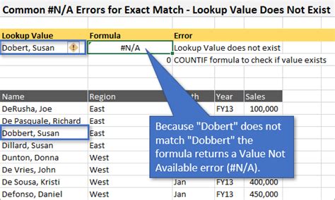
Mastering VLOOKUP with two Excel workbooks can seem daunting, but with practice and patience, you can become proficient in using this powerful function. Remember to use the correct syntax, specify exact or approximate matches, and troubleshoot common errors. By following the methods outlined in this article, you'll be able to efficiently retrieve data from one workbook to another and improve your productivity.

We hope you found this article helpful. If you have any questions or need further assistance, please don't hesitate to ask. Share your thoughts and experiences with VLOOKUP in the comments below.