Match Data In Two Excel Sheets With Ease

When working with large datasets in Excel, it's not uncommon to have data spread across multiple sheets. In such cases, matching data between two Excel sheets can be a daunting task, especially if you're dealing with thousands of rows. However, with the right techniques and tools, you can accomplish this task with ease.

In this article, we'll explore the various methods to match data in two Excel sheets, including using formulas, pivot tables, and add-ins. We'll also discuss the benefits and limitations of each approach, so you can choose the best method for your specific needs.

Why Match Data in Excel Sheets?

Before we dive into the methods, let's briefly discuss why matching data in Excel sheets is important. Here are a few scenarios where data matching is crucial:

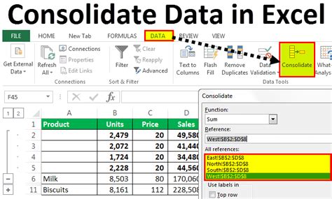
• Data consolidation: When you have data scattered across multiple sheets, you may need to consolidate it into a single sheet for analysis or reporting purposes.
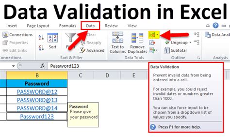
• Data validation: Matching data between sheets helps ensure data accuracy and consistency, which is critical in applications like accounting, finance, or scientific research.
• Data analysis: By matching data between sheets, you can perform more comprehensive analysis, identify trends, and make informed decisions.

Method 1: Using VLOOKUP Formula

One of the most common methods to match data in Excel sheets is by using the VLOOKUP formula. This formula allows you to search for a value in a table and return a corresponding value from another column.

To use VLOOKUP, follow these steps:

1. Open your Excel workbook and select the sheet that contains the data you want to match.
2. In the cell where you want to display the matched data, enter the VLOOKUP formula: =VLOOKUP(lookup_value, table_array, col_index_num, [range_lookup])
3. The lookup_value is the value you want to search for, table_array is the range of cells that contains the data you want to search, col_index_num is the column number that contains the data you want to return, and [range_lookup] is an optional argument that specifies whether you want an exact match or an approximate match.
4. Press Enter to execute the formula.

Example:

Suppose you have two sheets, "Sheet1" and "Sheet2", with the following data:

ID	Name	Age
1	John	25
2	Mary	31
3	David	42

ID	Department
1	Sales
2	Marketing
3	IT

To match the data in Sheet1 with the data in Sheet2, you can use the VLOOKUP formula:

=VLOOKUP(A2, Sheet2!A:B, 2, FALSE)

This formula searches for the value in cell A2 (ID) in the first column of the range A:B in Sheet2 and returns the corresponding value in the second column (Department).

Method 2: Using INDEX-MATCH Formula

Another powerful method to match data in Excel sheets is by using the INDEX-MATCH formula combination. This method is more flexible and efficient than VLOOKUP, especially when working with large datasets.

To use INDEX-MATCH, follow these steps:

1. Open your Excel workbook and select the sheet that contains the data you want to match.
2. In the cell where you want to display the matched data, enter the INDEX-MATCH formula: =INDEX(range, MATCH(lookup_value, lookup_array, [match_type])
3. The range is the range of cells that contains the data you want to return, lookup_value is the value you want to search for, lookup_array is the range of cells that contains the values you want to search, and [match_type] is an optional argument that specifies the match type.
4. Press Enter to execute the formula.

Example:

Using the same data as before, you can use the INDEX-MATCH formula to match the data in Sheet1 with the data in Sheet2:

=INDEX(Sheet2!B:B, MATCH(A2, Sheet2!A:A, 0))

This formula searches for the value in cell A2 (ID) in the first column of the range A:A in Sheet2 and returns the corresponding value in the second column (Department).

Method 3: Using Pivot Tables

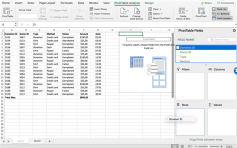
Pivot tables are a powerful tool in Excel that allows you to summarize and analyze large datasets. You can use pivot tables to match data between two sheets by creating a pivot table that links to both sheets.

To use pivot tables, follow these steps:

1. Open your Excel workbook and select the sheet that contains the data you want to match.
2. Go to the "Insert" tab and click on "PivotTable".
3. Select the range of cells that contains the data you want to match and click "OK".
4. In the "PivotTable Fields" pane, drag the field that contains the values you want to match to the "Row Labels" area.
5. Drag the field that contains the values you want to return to the "Values" area.
6. Right-click on the pivot table and select "PivotTable Options".
7. In the "PivotTable Options" dialog box, click on the "Data" tab and select the sheet that contains the data you want to match.
8. Click "OK" to close the dialog box.

Example:

Using the same data as before, you can create a pivot table that links to both Sheet1 and Sheet2:

1. Select the range A1:C3 in Sheet1 and create a pivot table.
2. Drag the "ID" field to the "Row Labels" area.
3. Drag the "Department" field to the "Values" area.
4. Right-click on the pivot table and select "PivotTable Options".
5. In the "PivotTable Options" dialog box, click on the "Data" tab and select Sheet2.
6. Click "OK" to close the dialog box.

The pivot table will display the matched data from both sheets.

Method 4: Using Add-ins

There are several add-ins available that can help you match data in Excel sheets, such as Power Query, Power Pivot, and Excel add-ins like AutoMate or Excel- SQL.

These add-ins provide more advanced features and functionalities than the built-in Excel formulas and pivot tables, but they may require additional installation and configuration.

Conclusion

Matching data in two Excel sheets can be a challenging task, but with the right techniques and tools, you can accomplish it with ease. Whether you use VLOOKUP, INDEX-MATCH, pivot tables, or add-ins, the key is to understand the strengths and limitations of each method and choose the best approach for your specific needs.

Remember to always validate your data and ensure that it is accurate and consistent before performing any data matching or analysis.

Image Gallery:

Excel Data Matching Image Gallery

FAQ

Q: What is the best method to match data in Excel sheets? A: The best method depends on the size and complexity of your data, as well as your personal preference. VLOOKUP and INDEX-MATCH are popular formulas, while pivot tables and add-ins offer more advanced features.

Q: Can I use multiple criteria to match data in Excel? A: Yes, you can use multiple criteria to match data in Excel using formulas like VLOOKUP and INDEX-MATCH, or by using pivot tables with multiple fields.

Q: How do I ensure data accuracy and consistency when matching data in Excel? A: Always validate your data and ensure that it is accurate and consistent before performing any data matching or analysis.

Q: Can I use Excel add-ins to match data in Excel sheets? A: Yes, there are several Excel add-ins available that can help you match data in Excel sheets, such as Power Query, Power Pivot, and Excel- SQL.