
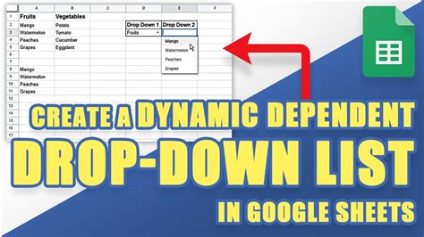
Google Sheets is a powerful tool for data analysis and visualization, and one of its most useful features is the ability to create dynamic drop-down lists. A dynamic drop-down list is a list of options that changes based on the selection made in another cell or list. In this article, we will explore five ways to create dynamic drop-down lists in Google Sheets.
Why Use Dynamic Drop-Down Lists in Google Sheets?
Dynamic drop-down lists are useful in a variety of situations, such as:
- Creating a form that changes based on user input
- Building a dashboard that updates based on selection
- Creating a list of options that changes based on data in another sheet
- Simplifying data entry by providing a list of valid options
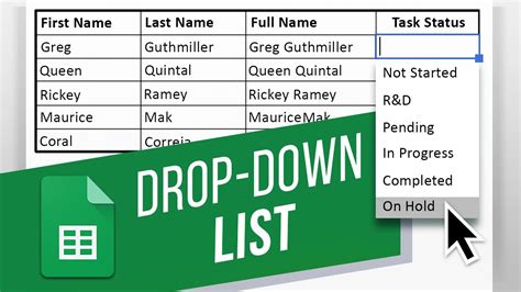
Method 1: Using the Data Validation Feature
The data validation feature in Google Sheets allows you to create a drop-down list that changes based on the selection made in another cell. To create a dynamic drop-down list using data validation, follow these steps:
- Select the cell where you want to create the drop-down list
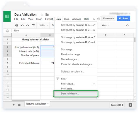
- Go to the "Data" menu and select "Data validation"
- Select "List of items" from the drop-down menu
- Enter the range of cells that contains the list of options
- Check the box next to "Show dropdown list in cell"
- Click "Save"
Example:
Suppose you have a sheet with a list of countries in column A, and you want to create a drop-down list of cities in column B that changes based on the country selected in column A. You can use the data validation feature to create a dynamic drop-down list.
| Country | City |
|---|---|
| USA | New York |
| USA | Los Angeles |
| Canada | Toronto |
| Canada | Vancouver |
To create the dynamic drop-down list, select cell B2 and follow the steps above. Enter the range of cells A2:A5 in the "List of items" field, and check the box next to "Show dropdown list in cell". When you select a country in cell A2, the list of cities in cell B2 will change accordingly.
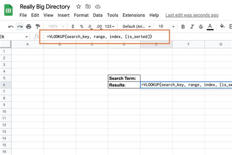
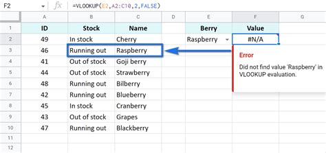
Method 2: Using the VLOOKUP Function
The VLOOKUP function in Google Sheets allows you to look up a value in a table and return a corresponding value from another column. You can use the VLOOKUP function to create a dynamic drop-down list that changes based on the selection made in another cell.
Example:
Suppose you have a sheet with a list of products in column A, and a list of prices in column B. You want to create a drop-down list of prices in cell C2 that changes based on the product selected in cell A2. You can use the VLOOKUP function to create a dynamic drop-down list.
| Product | Price |
|---|---|
| Product A | $10 |
| Product B | $20 |
| Product C | $30 |
To create the dynamic drop-down list, enter the following formula in cell C2:
=VLOOKUP(A2, A:B, 2, FALSE)
This formula looks up the value in cell A2 in the first column of the range A:B, and returns the corresponding value in the second column. When you select a product in cell A2, the price in cell C2 will change accordingly.
Method 3: Using the INDEX/MATCH Function
The INDEX/MATCH function in Google Sheets is a more powerful and flexible alternative to the VLOOKUP function. You can use the INDEX/MATCH function to create a dynamic drop-down list that changes based on the selection made in another cell.
Example:
Suppose you have a sheet with a list of products in column A, and a list of prices in column B. You want to create a drop-down list of prices in cell C2 that changes based on the product selected in cell A2. You can use the INDEX/MATCH function to create a dynamic drop-down list.
| Product | Price |
|---|---|
| Product A | $10 |
| Product B | $20 |
| Product C | $30 |
To create the dynamic drop-down list, enter the following formula in cell C2:
=INDEX(B:B, MATCH(A2, A:A, 0))
This formula looks up the value in cell A2 in the range A:A, and returns the corresponding value in the range B:B. When you select a product in cell A2, the price in cell C2 will change accordingly.
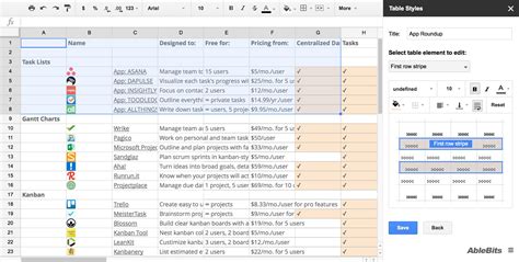
Method 4: Using Google Sheets Add-ons
There are several Google Sheets add-ons available that can help you create dynamic drop-down lists. One popular add-on is "Dynamic Dropdowns" which allows you to create dynamic drop-down lists based on the selection made in another cell.
Example:
Suppose you have a sheet with a list of countries in column A, and you want to create a drop-down list of cities in column B that changes based on the country selected in column A. You can use the Dynamic Dropdowns add-on to create a dynamic drop-down list.
To use the add-on, follow these steps:
- Go to the Google Sheets add-on store and install the Dynamic Dropdowns add-on
- Select the cell where you want to create the drop-down list
- Click on the "Dynamic Dropdowns" button in the toolbar
- Select the range of cells that contains the list of options
- Check the box next to "Show dropdown list in cell"
- Click "Save"
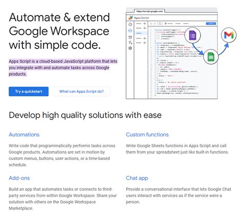
Method 5: Using Google Apps Script
Google Apps Script is a powerful tool that allows you to automate tasks in Google Sheets. You can use Google Apps Script to create dynamic drop-down lists that change based on the selection made in another cell.
Example:
Suppose you have a sheet with a list of products in column A, and a list of prices in column B. You want to create a drop-down list of prices in cell C2 that changes based on the product selected in cell A2. You can use Google Apps Script to create a dynamic drop-down list.
To create the dynamic drop-down list, follow these steps:
- Go to the "Tools" menu and select "Script editor"
- Create a new function that looks up the value in cell A2 and returns the corresponding value in cell C2
- Use the
getRange()andsetValue()methods to update the value in cell C2 - Save the script and deploy it as a web app
Dynamic Drop-Down Lists in Google Sheets Image Gallery
We hope this article has helped you learn how to create dynamic drop-down lists in Google Sheets. Whether you use the data validation feature, the VLOOKUP function, the INDEX/MATCH function, Google Sheets add-ons, or Google Apps Script, you can create powerful and flexible drop-down lists that make your data analysis and visualization tasks easier and more efficient.