
Intro
Discover the power of Excels Conditional Formatting feature. Learn 5 easy ways to highlight rows in Excel, including using formulas, values, and formatting rules. Master conditional formatting techniques to streamline your workflow, identify trends, and visualize data. Unlock efficient data analysis and presentation with this step-by-step guide.
Excel is a powerful tool for data analysis, and one of its most useful features is conditional formatting. This feature allows you to highlight cells or rows based on specific conditions, making it easier to visualize and understand your data. In this article, we'll explore five ways to highlight rows in Excel using conditional formatting.
What is Conditional Formatting?
Conditional formatting is a feature in Excel that allows you to apply formatting to cells or rows based on specific conditions. You can use formulas, values, or formatting rules to determine which cells or rows to format. This feature is useful for highlighting trends, patterns, and anomalies in your data.
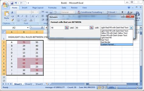
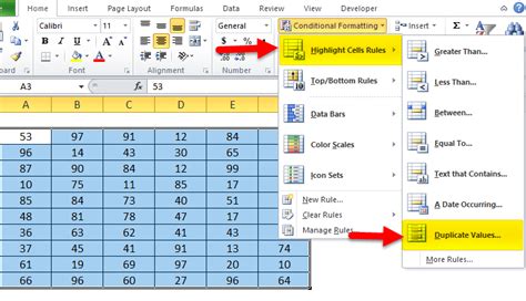
Method 1: Highlighting Rows Based on a Value
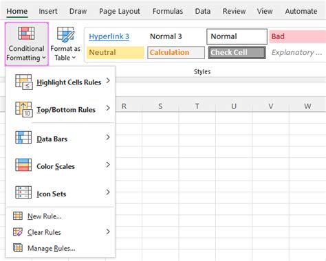
One of the simplest ways to highlight rows in Excel is to use the "Highlight Cells Rules" feature. This feature allows you to highlight cells or rows based on a specific value or condition.

To use this feature, follow these steps:
- Select the range of cells you want to format
- Go to the "Home" tab in the Excel ribbon
- Click on the "Conditional Formatting" button in the "Styles" group
- Select "Highlight Cells Rules" from the drop-down menu
- Choose the type of rule you want to apply (e.g. "Greater Than", "Less Than", etc.)
- Enter the value or condition you want to use to highlight the cells
- Click "OK" to apply the formatting
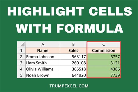
Method 2: Highlighting Rows Based on a Formula
Another way to highlight rows in Excel is to use a formula to determine which rows to format. This method is useful when you need to highlight rows based on a complex condition.
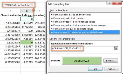
To use this method, follow these steps:
- Select the range of cells you want to format
- Go to the "Home" tab in the Excel ribbon
- Click on the "Conditional Formatting" button in the "Styles" group
- Select "New Rule" from the drop-down menu
- Choose "Use a formula to determine which cells to format"
- Enter the formula you want to use to highlight the cells
- Click "OK" to apply the formatting
Method 3: Highlighting Rows Based on a Format
You can also highlight rows in Excel based on a specific format. For example, you can highlight rows that contain a specific font, color, or alignment.
To use this method, follow these steps:
- Select the range of cells you want to format
- Go to the "Home" tab in the Excel ribbon
- Click on the "Conditional Formatting" button in the "Styles" group
- Select "Format Values Where This Formula Is True"
- Choose the format you want to use to highlight the cells
- Click "OK" to apply the formatting
Method 4: Highlighting Rows Based on a Data Validation Rule
Data validation rules allow you to restrict the data that can be entered into a cell or range of cells. You can also use data validation rules to highlight rows in Excel.

To use this method, follow these steps:
- Select the range of cells you want to format
- Go to the "Data" tab in the Excel ribbon
- Click on the "Data Validation" button in the "Data Tools" group
- Select "Settings" from the drop-down menu
- Choose the type of data validation rule you want to apply (e.g. "Whole Number", "Date", etc.)
- Enter the criteria for the data validation rule
- Click "OK" to apply the rule
- Go to the "Home" tab and click on the "Conditional Formatting" button
- Select "Highlight Cells Rules" from the drop-down menu
- Choose "Data Validation Rule" from the list of rules
- Click "OK" to apply the formatting
Method 5: Highlighting Rows Using a Macro
Finally, you can also highlight rows in Excel using a macro. Macros are small programs that automate repetitive tasks in Excel.

To use this method, follow these steps:
- Open the Visual Basic Editor by pressing "Alt + F11" or by navigating to the "Developer" tab and clicking on the "Visual Basic" button
- In the Visual Basic Editor, click on "Insert" and then "Module" to insert a new module
- Paste the following code into the module:
Sub HighlightRows()
    Dim rng As Range
    Set rng = Selection
    rng.Interior.ColorIndex = 6
End Sub
- Click "Run" to run the macro
- Select the range of cells you want to format
- Run the macro again to highlight the rows
Gallery of Conditional Formatting Examples


Conclusion:
In this article, we explored five ways to highlight rows in Excel using conditional formatting. Whether you need to highlight rows based on a value, formula, format, data validation rule, or macro, Excel provides a range of tools to help you achieve your goals. By mastering these techniques, you can take your data analysis to the next level and gain a deeper understanding of your data.