Intro
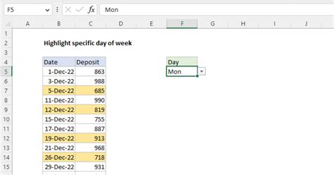
Master the art of highlighting specific days of the week in Excel using conditional formatting. Learn how to emphasize important dates, such as weekends, weekdays, or specific days like Mondays or Fridays. Discover techniques to apply different formats, like colors, fonts, and icons, to create visually appealing and informative spreadsheets.
Highlighting specific days of the week in a dataset can help identify patterns, trends, and correlations. Excel's conditional formatting feature is an excellent tool for this task. By applying conditional formatting, you can visually distinguish specific days of the week, making it easier to analyze and understand your data.
Benefits of Highlighting Days of the Week in Excel

Highlighting specific days of the week in Excel can:
- Help identify peak sales days or seasons
- Reveal patterns in employee work schedules or attendance
- Facilitate planning and organization for events or appointments
- Enhance data visualization and readability
- Support data-driven decision-making
Step-by-Step Guide to Highlighting Days of the Week in Excel

To highlight specific days of the week in Excel, follow these steps:
Step 1: Prepare Your Data
- Ensure your data is in a table format with dates in a single column.
- Use the
TEXTfunction to extract the day of the week from the date column, if needed.
Step 2: Select the Data Range
- Choose the cell range that contains the dates you want to format.
Step 3: Apply Conditional Formatting
- Go to the "Home" tab in the Excel ribbon.
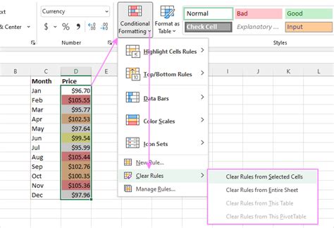
- Click on the "Conditional Formatting" button in the "Styles" group.
- Select "New Rule" from the drop-down menu.
- Choose "Use a formula to determine which cells to format."
- Enter the formula:
=WEEKDAY(A1,2)=1(assuming the date is in cell A1 and you want to highlight Mondays). - Click "Format" and select the desired format (e.g., fill color, font color).
- Click "OK" to apply the rule.
Step 4: Modify the Formula for Different Days
- To highlight different days, modify the formula accordingly:
- Monday:
=WEEKDAY(A1,2)=1 - Tuesday:
=WEEKDAY(A1,2)=2 - Wednesday:
=WEEKDAY(A1,2)=3 - Thursday:
=WEEKDAY(A1,2)=4 - Friday:
=WEEKDAY(A1,2)=5 - Saturday:
=WEEKDAY(A1,2)=6 - Sunday:
=WEEKDAY(A1,2)=7
- Monday:
Step 5: Apply the Rule to the Entire Data Range
- Select the entire data range that you want to apply the formatting to.
- Go to the "Home" tab and click on the "Conditional Formatting" button.
- Select "Manage Rules" from the drop-down menu.
- Find the rule you created earlier and click "Apply."
Example Use Case: Highlighting Peak Sales Days

Suppose you have a dataset with daily sales figures and you want to highlight the days with the highest sales (e.g., Fridays and Saturdays). You can apply the conditional formatting rule to highlight these days and quickly identify patterns in your sales data.
Step 6: Customize the Formatting Options
- To customize the formatting options, go to the "Home" tab and click on the "Conditional Formatting" button.
- Select "Manage Rules" from the drop-down menu.
- Find the rule you created earlier and click "Edit Rule."
- Modify the formatting options as desired (e.g., change the fill color or font style).
Step 7: Apply the Rule to Other Data Ranges
- To apply the same rule to other data ranges, select the new data range and go to the "Home" tab.
- Click on the "Conditional Formatting" button and select "Manage Rules" from the drop-down menu.
- Find the rule you created earlier and click "Apply."
Step 8: Troubleshoot Common Issues
- If the formatting rule is not working as expected, check the following:
- Ensure the formula is correct and the date format is consistent.
- Verify that the rule is applied to the correct data range.
- Check for any conflicting formatting rules.
Best Practices for Using Conditional Formatting in Excel

To get the most out of conditional formatting in Excel, follow these best practices:
- Use clear and concise formulas to avoid errors.
- Apply formatting rules to specific data ranges to avoid unnecessary formatting.
- Use consistent formatting options throughout your workbook.
- Test and troubleshoot your formatting rules to ensure they work as expected.
Common Mistakes to Avoid When Using Conditional Formatting

When using conditional formatting in Excel, avoid the following common mistakes:
- Incorrect formula syntax or logic.
- Applying formatting rules to incorrect data ranges.
- Not testing or troubleshooting formatting rules.
- Using inconsistent formatting options.
- Not documenting or commenting on formatting rules.
Gallery of Excel Conditional Formatting Examples
Excel Conditional Formatting Examples


Conclusion
Highlighting specific days of the week in Excel can be a powerful tool for data analysis and visualization. By following the steps outlined in this article, you can apply conditional formatting rules to highlight specific days and gain insights into your data. Remember to use clear and concise formulas, apply formatting rules to specific data ranges, and test and troubleshoot your formatting rules to ensure they work as expected.
Final Thoughts
- Practice makes perfect. Experiment with different conditional formatting rules to become more comfortable with the feature.
- Share your knowledge with others. Teach your colleagues or friends how to use conditional formatting in Excel.
- Stay up-to-date with the latest Excel features and updates. Microsoft regularly releases new features and improvements to Excel.
- Join online communities or forums to connect with other Excel users and learn from their experiences.
- Don't be afraid to ask for help. If you're struggling with a specific formatting rule or feature, don't hesitate to reach out to a colleague or online community for assistance.
