Intro
Boost your Excel skills with Rank.Eq! Discover 5 powerful ways to utilize this function, from ranking numbers to evaluating data. Learn how to use Rank.Eq with IF statements, arrays, and more. Master data analysis, comparisons, and sorting with this versatile function. Improve your spreadsheet game with these expert tips and tricks.
Excel is an incredibly powerful tool for data analysis, and one of its most useful functions is the RANK.EQ function. This function allows you to rank numbers in a list based on their value, and it's especially useful when you need to compare values in a dataset. In this article, we'll explore five ways to use the RANK.EQ function in Excel, along with some practical examples to help you get started.
What is the RANK.EQ Function?

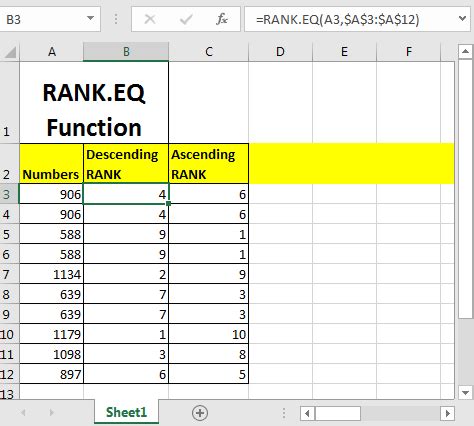
The RANK.EQ function is a statistical function in Excel that returns the rank of a number in a list of numbers. It's similar to the RANK function, but it uses an "equivalent" ranking method, which means that if two or more values are equal, they will receive the same rank. The RANK.EQ function is available in Excel 2010 and later versions.
Syntax of the RANK.EQ Function
The syntax of the RANK.EQ function is as follows:
RANK.EQ(number,ref,[order])
- number: The number for which you want to find the rank.
- ref: The array of numbers that contains the values to be ranked.
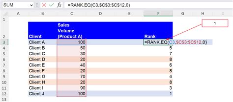
- order: Optional. A value that specifies how to rank the numbers. If order is 0 (zero) or omitted, the numbers are ranked in descending order. If order is any non-zero value, the numbers are ranked in ascending order.
1. Ranking Student Grades
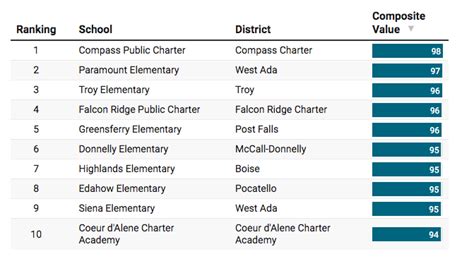
Suppose you have a list of student grades in a class, and you want to rank them based on their scores. You can use the RANK.EQ function to do this.
| Student | Grade |
|---|---|
| John | 85 |
| Mary | 90 |
| Jane | 78 |
| Bob | 92 |
| Alice | 85 |
To rank the grades, you can use the following formula:
=RANK.EQ(B2,$B$2:$B$6,0)
Assuming the grades are in cells B2:B6, this formula will return the rank of each grade in descending order.
Result
| Student | Grade | Rank |
|---|---|---|
| John | 85 | 3 |
| Mary | 90 | 2 |
| Jane | 78 | 5 |
| Bob | 92 | 1 |
| Alice | 85 | 3 |
As you can see, John and Alice have the same rank (3) because they have the same grade (85).
2. Ranking Sales Performance
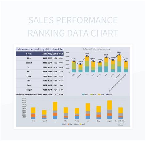
Suppose you have a list of sales data for a company, and you want to rank the sales performance of each region. You can use the RANK.EQ function to do this.
| Region | Sales |
|---|---|
| North | 1000 |
| South | 800 |
| East | 1200 |
| West | 900 |
To rank the sales performance, you can use the following formula:
=RANK.EQ(B2,$B$2:$B$5,0)
Assuming the sales data is in cells B2:B5, this formula will return the rank of each region's sales performance in descending order.
Result
| Region | Sales | Rank |
|---|---|---|
| North | 1000 | 2 |
| South | 800 | 4 |
| East | 1200 | 1 |
| West | 900 | 3 |
As you can see, the East region has the highest sales performance (rank 1), and the South region has the lowest sales performance (rank 4).
3. Ranking Website Traffic

Suppose you have a list of website traffic data, and you want to rank the traffic of each webpage. You can use the RANK.EQ function to do this.
| Webpage | Traffic |
|---|---|
| Home | 10000 |
| About | 5000 |
| Contact | 2000 |
| Blog | 8000 |
To rank the traffic, you can use the following formula:
=RANK.EQ(B2,$B$2:$B$5,0)
Assuming the traffic data is in cells B2:B5, this formula will return the rank of each webpage's traffic in descending order.
Result
| Webpage | Traffic | Rank |
|---|---|---|
| Home | 10000 | 1 |
| About | 5000 | 3 |
| Contact | 2000 | 4 |
| Blog | 8000 | 2 |
As you can see, the Home webpage has the highest traffic (rank 1), and the Contact webpage has the lowest traffic (rank 4).
4. Ranking Employee Performance

Suppose you have a list of employee performance data, and you want to rank the performance of each employee. You can use the RANK.EQ function to do this.
| Employee | Performance |
|---|---|
| John | 85 |
| Mary | 90 |
| Jane | 78 |
| Bob | 92 |
| Alice | 85 |
To rank the performance, you can use the following formula:
=RANK.EQ(B2,$B$2:$B$6,0)
Assuming the performance data is in cells B2:B6, this formula will return the rank of each employee's performance in descending order.
Result
| Employee | Performance | Rank |
|---|---|---|
| John | 85 | 3 |
| Mary | 90 | 2 |
| Jane | 78 | 5 |
| Bob | 92 | 1 |
| Alice | 85 | 3 |
As you can see, Bob has the highest performance (rank 1), and Jane has the lowest performance (rank 5).
5. Ranking Sports Teams

Suppose you have a list of sports teams, and you want to rank their performance based on their wins and losses. You can use the RANK.EQ function to do this.
| Team | Wins | Losses |
|---|---|---|
| Team A | 10 | 2 |
| Team B | 8 | 4 |
| Team C | 12 | 1 |
| Team D | 6 | 6 |
To rank the teams, you can use the following formula:
=RANK.EQ(B2,$B$2:$B$5,0)
Assuming the wins data is in cells B2:B5, this formula will return the rank of each team's performance in descending order.
Result
| Team | Wins | Losses | Rank |
|---|---|---|---|
| Team A | 10 | 2 | 2 |
| Team B | 8 | 4 | 4 |
| Team C | 12 | 1 | 1 |
| Team D | 6 | 6 | 3 |
As you can see, Team C has the highest performance (rank 1), and Team B has the lowest performance (rank 4).
Rank.EQ Function Image Gallery






We hope this article has helped you understand how to use the RANK.EQ function in Excel. With its ability to rank numbers in a list based on their value, this function is a powerful tool for data analysis. Whether you're ranking student grades, sales performance, website traffic, employee performance, or sports teams, the RANK.EQ function can help you make sense of your data. Try it out today and see how it can help you make better decisions!
