Intro
Master data analysis with ease! Learn 5 powerful ways to use Index Match functions across multiple sheets in Excel. Discover how to perform lookups, retrieve data, and automate tasks efficiently using this versatile formula. Boost productivity and accuracy with these expert-approved techniques and take your data manipulation skills to the next level.
In the world of data analysis, working with multiple sheets in a single workbook is a common scenario. One of the most powerful and flexible ways to manipulate data across multiple sheets is by using the INDEX-MATCH function combination. In this article, we will explore five ways to use INDEX-MATCH across multiple sheets, making you a master of data analysis in no time.
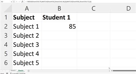
Understanding INDEX-MATCH
Before diving into the various ways to use INDEX-MATCH across multiple sheets, it's essential to understand the basics of this function combination. INDEX-MATCH is a powerful alternative to VLOOKUP, allowing you to perform lookups in any direction, not just from left to right.
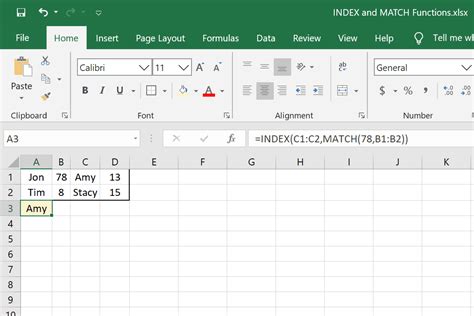
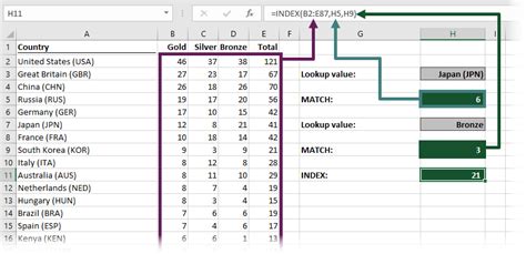
The INDEX function returns a value at a specified position in a range or array. The MATCH function returns the relative position of a value within a range or array. When combined, INDEX-MATCH can perform lookups, retrieve data, and even handle multiple criteria.
Basic Syntax of INDEX-MATCH
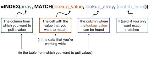
The basic syntax of INDEX-MATCH is as follows:
=INDEX(range, MATCH(lookup_value, lookup_array, [match_type])
rangeis the range of cells that contains the value you want to return.lookup_valueis the value you want to look up.lookup_arrayis the range of cells that contains the values you want to search.match_typeis an optional argument that specifies the match type (exact, less than, greater than, etc.).
Method 1: Basic INDEX-MATCH Across Multiple Sheets
In this example, we will use INDEX-MATCH to retrieve data from a different sheet.
Suppose we have two sheets, "Sales" and "Products." We want to retrieve the product name from the "Products" sheet based on the product ID in the "Sales" sheet.
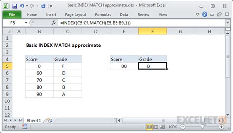
The formula would be:
=INDEX(Products!A:A, MATCH(Sales!A2, Products!B:B, 0))
In this formula, we are looking up the value in cell A2 of the "Sales" sheet in the range B:B of the "Products" sheet. The MATCH function returns the relative position of the value, which is then used by the INDEX function to return the corresponding product name from range A:A.
Method 2: Using INDEX-MATCH with Multiple Criteria
In this example, we will use INDEX-MATCH to retrieve data from a different sheet based on multiple criteria.
Suppose we have two sheets, "Sales" and "Products." We want to retrieve the product name from the "Products" sheet based on the product ID and category in the "Sales" sheet.
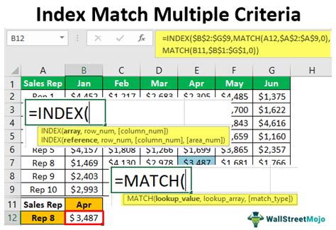
The formula would be:
=INDEX(Products!A:A, MATCH(1, (Sales!A2=Products!B:B) * (Sales!B2=Products!C:C), 0))
In this formula, we are using the MATCH function with multiple criteria. The first criteria is the product ID, and the second criteria is the category. The * operator is used to multiply the two criteria, and the 1 at the beginning of the MATCH function is used to find the first occurrence of the value.
Method 3: Using INDEX-MATCH with Dynamic Ranges
In this example, we will use INDEX-MATCH to retrieve data from a different sheet based on dynamic ranges.
Suppose we have two sheets, "Sales" and "Products." We want to retrieve the product name from the "Products" sheet based on the product ID in the "Sales" sheet, and we want to dynamically adjust the range based on the number of rows in the "Products" sheet.
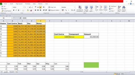
The formula would be:
=INDEX(Products!A:A, MATCH(Sales!A2, OFFSET(Products!B:B, 0, 0, COUNTA(Products!B:B), 1), 0))
In this formula, we are using the OFFSET function to dynamically adjust the range based on the number of rows in the "Products" sheet. The COUNTA function is used to count the number of rows in the "Products" sheet, and the OFFSET function is used to adjust the range accordingly.
Method 4: Using INDEX-MATCH with Arrays
In this example, we will use INDEX-MATCH to retrieve data from a different sheet based on arrays.
Suppose we have two sheets, "Sales" and "Products." We want to retrieve the product name from the "Products" sheet based on the product ID in the "Sales" sheet, and we want to return multiple values using arrays.

The formula would be:
=INDEX(Products!A:A, N(IF(Sales!A2=Products!B:B, ROW(Products!B:B)-ROW(Products!B1)+1)))
In this formula, we are using the IF function to create an array of values based on the product ID. The N function is used to convert the array to a numerical value, and the ROW function is used to return the relative position of the value.
Method 5: Using INDEX-MATCH with Named Ranges
In this example, we will use INDEX-MATCH to retrieve data from a different sheet based on named ranges.
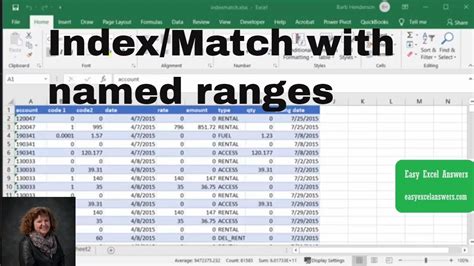
Suppose we have two sheets, "Sales" and "Products." We want to retrieve the product name from the "Products" sheet based on the product ID in the "Sales" sheet, and we want to use named ranges to make the formula more readable.
The formula would be:
=INDEX(Product_Names, MATCH(Sales_Product_ID, Product_IDs, 0))
In this formula, we are using named ranges to make the formula more readable. The Product_Names range refers to the range of product names in the "Products" sheet, and the Product_IDs range refers to the range of product IDs in the "Products" sheet.
Index Match Image Gallery



Now that you've mastered the five ways to use INDEX-MATCH across multiple sheets, it's time to put your skills to the test! Try using these methods in your own worksheets and see how they can help you streamline your data analysis tasks. Don't forget to share your experiences and tips with others in the comments below.
