Year To Date Formula In Excel Made Easy

The Year To Date (YTD) formula in Excel is a powerful tool for financial analysis, accounting, and business planning. It helps to calculate the total value of a particular metric or data point from the beginning of the year up to a specific date, making it easier to track progress, identify trends, and make informed decisions.

The YTD formula is commonly used in various industries, including finance, accounting, and business management. It is particularly useful for calculating the total sales, revenue, expenses, or profits for a specific period within a year.

In this article, we will explore the YTD formula in Excel, including its syntax, usage, and examples. We will also provide step-by-step instructions on how to apply the formula to real-world scenarios.

Understanding the YTD Formula

The YTD formula in Excel is used to calculate the total value of a data point from the beginning of the year up to a specific date. The formula takes into account the year and date of the data point, and returns the total value from the beginning of the year to the specified date.

The basic syntax of the YTD formula is:

=SUMIFS(data_range, date_range, ">="&DATE(YEAR(date), 1, 1), date_range, "<="&date)

Where:

• data_range is the range of cells containing the data to be summed.
• date_range is the range of cells containing the dates to be considered.
• date is the specific date for which the YTD value is to be calculated.

How to Use the YTD Formula

To use the YTD formula in Excel, follow these steps:

1. Select the cell where you want to display the YTD value.
2. Enter the YTD formula using the syntax above.
3. Press Enter to calculate the formula.

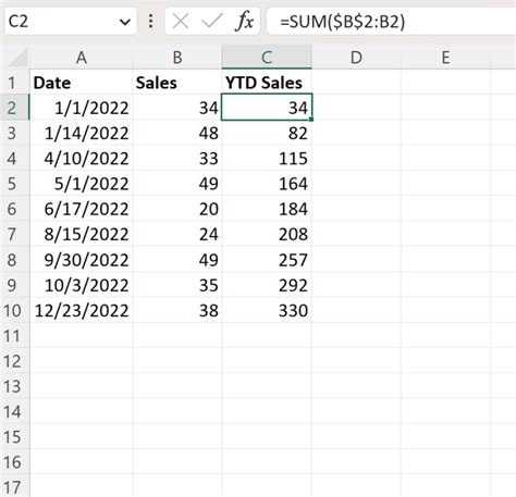
For example, let's say we have a data range A1:B12 containing sales data for the year 2022, where column A contains the dates and column B contains the sales amounts. We want to calculate the YTD sales for March 31, 2022.

=SUMIFS(B:B, A:A, ">="&DATE(2022, 1, 1), A:A, "<="&DATE(2022, 3, 31))

This formula will return the total sales from January 1, 2022, to March 31, 2022.

Image:

Using the YTD Formula with Multiple Criteria

The YTD formula can also be used with multiple criteria to filter the data. For example, let's say we want to calculate the YTD sales for a specific region.

=SUMIFS(B:B, A:A, ">="&DATE(2022, 1, 1), A:A, "<="&DATE(2022, 3, 31), C:C, "North")

This formula will return the total sales for the North region from January 1, 2022, to March 31, 2022.

Image:

Tips and Variations

Here are some tips and variations for using the YTD formula in Excel:

• Use the YEAR function to extract the year from a date.
• Use the DATE function to create a date from a year, month, and day.
• Use the SUMIFS function to sum data based on multiple criteria.
• Use the SUMIF function to sum data based on a single criterion.
• Use the EOMONTH function to calculate the last day of a month.

Gallery of YTD Formula Examples

YTD Formula Image Gallery

Conclusion

The YTD formula in Excel is a powerful tool for financial analysis and business planning. By using the SUMIFS function and the DATE function, you can calculate the total value of a data point from the beginning of the year up to a specific date. We hope this article has helped you to understand the YTD formula and how to use it in your Excel spreadsheets. If you have any questions or need further assistance, please don't hesitate to comment below.