Looking up text in Excel can be a daunting task, especially when dealing with large datasets. However, Excel provides several methods to make this process easier and more efficient. In this article, we will explore five ways to lookup text in Excel, including using formulas, functions, and shortcuts.
The Importance of Lookup Functions in Excel
Lookup functions in Excel are essential for data analysis and manipulation. They enable users to search for specific values within a dataset and return corresponding data. This is particularly useful when working with large datasets or when data is scattered across multiple sheets or workbooks.
Method 1: Using the VLOOKUP Function

The VLOOKUP function is one of the most commonly used lookup functions in Excel. It searches for a value in the first column of a table and returns a value in the same row from another column.
The syntax for the VLOOKUP function is:
VLOOKUP(lookup_value, table_array, col_index_num, [range_lookup])
- lookup_value: The value to be searched for.
- table_array: The range of cells that contains the data to be searched.
- col_index_num: The column number that contains the value to be returned.
- [range_lookup]: Optional. If TRUE, the function will perform an approximate match. If FALSE, the function will perform an exact match.
For example, suppose we have a table with employee names in column A and their corresponding departments in column B. We can use the VLOOKUP function to find the department of a specific employee.
Example: Using VLOOKUP to Find Employee Department
| Employee Name | Department |
|---|---|
| John Smith | Sales |
| Jane Doe | Marketing |
| Bob Johnson | IT |
Using the VLOOKUP function, we can find the department of John Smith as follows:
VLOOKUP("John Smith", A:B, 2, FALSE)
This will return "Sales" as the department of John Smith.
Method 2: Using the INDEX-MATCH Function

The INDEX-MATCH function is a more flexible and powerful alternative to the VLOOKUP function. It uses the INDEX function to return a value at a specified position in a range, based on a match found by the MATCH function.
The syntax for the INDEX-MATCH function is:
INDEX(range, MATCH(lookup_value, lookup_array, [match_type]))
- range: The range of cells that contains the data to be searched.
- lookup_value: The value to be searched for.
- lookup_array: The range of cells that contains the values to be searched.
- [match_type]: Optional. If 0, the function will perform an exact match. If 1, the function will perform a less-than match. If -1, the function will perform a greater-than match.
For example, suppose we have a table with employee names in column A and their corresponding salaries in column B. We can use the INDEX-MATCH function to find the salary of a specific employee.
Example: Using INDEX-MATCH to Find Employee Salary
| Employee Name | Salary |
|---|---|
| John Smith | 50000 |
| Jane Doe | 60000 |
| Bob Johnson | 70000 |
Using the INDEX-MATCH function, we can find the salary of John Smith as follows:
INDEX(B:B, MATCH("John Smith", A:A, 0))
This will return 50000 as the salary of John Smith.
Method 3: Using the LOOKUP Function

The LOOKUP function is a simpler alternative to the VLOOKUP function. It searches for a value in a range and returns a corresponding value from another range.
The syntax for the LOOKUP function is:
LOOKUP(lookup_value, lookup_array, result_array)
- lookup_value: The value to be searched for.
- lookup_array: The range of cells that contains the values to be searched.
- result_array: The range of cells that contains the values to be returned.
For example, suppose we have a table with employee names in column A and their corresponding job titles in column B. We can use the LOOKUP function to find the job title of a specific employee.
Example: Using LOOKUP to Find Employee Job Title
| Employee Name | Job Title |
|---|---|
| John Smith | Sales Manager |
| Jane Doe | Marketing Manager |
| Bob Johnson | IT Manager |
Using the LOOKUP function, we can find the job title of John Smith as follows:
LOOKUP("John Smith", A:B, B:B)
This will return "Sales Manager" as the job title of John Smith.
Method 4: Using the FILTER Function

The FILTER function is a new function in Excel that allows users to filter a range of cells based on a condition.
The syntax for the FILTER function is:
FILTER(array, include, [if_empty])
- array: The range of cells that contains the data to be filtered.
- include: The condition to be applied to the data.
- [if_empty]: Optional. The value to be returned if the filtered range is empty.
For example, suppose we have a table with employee names in column A and their corresponding departments in column B. We can use the FILTER function to find the employees in a specific department.
Example: Using FILTER to Find Employees in a Specific Department
| Employee Name | Department |
|---|---|
| John Smith | Sales |
| Jane Doe | Marketing |
| Bob Johnson | IT |
Using the FILTER function, we can find the employees in the Sales department as follows:
FILTER(A:B, B:B = "Sales")
This will return the employees in the Sales department.
Method 5: Using Shortcuts

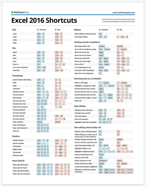
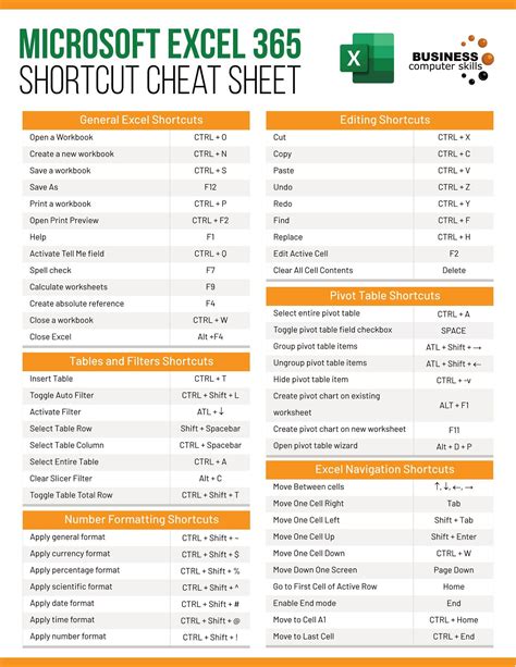
Excel provides several shortcuts that can be used to lookup text in a range. For example, the Ctrl + F shortcut can be used to open the Find and Replace dialog box, which allows users to search for a value in a range.
Another shortcut is the Ctrl + Shift + F shortcut, which can be used to open the Find and Replace dialog box with the "Find what" field selected.
Gallery of Excel Lookup Functions
Excel Lookup Functions Image Gallery


We hope this article has helped you learn about the different ways to lookup text in Excel. Whether you are using formulas, functions, or shortcuts, Excel provides a range of tools to make data analysis and manipulation easier and more efficient.
