Enter A Formula Using Averageifs In Excel

Entering a formula using AVERAGEIFS in Excel can be a powerful way to analyze data by averaging values based on multiple criteria. AVERAGEIFS is an extension of the AVERAGEIF function, which allows you to average values based on a single criterion. With AVERAGEIFS, you can apply multiple criteria across different ranges.

Understanding AVERAGEIFS

The AVERAGEIFS function in Excel averages cells in a range that meet multiple criteria. The syntax for AVERAGEIFS is:

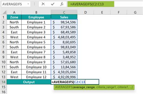
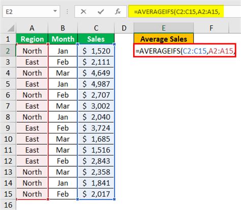
AVERAGEIFS(average_range, criteria_range1, criteria1, [criteria_range2], [criteria2],...)

• average_range: This is the range of cells that you want to average.
• criteria_range1: The first range of cells to apply the criteria to.
• criteria1: The first criterion that must be met.
• [criteria_range2], [criteria2],...: Additional ranges and criteria that you can apply.

Example of Using AVERAGEIFS

Suppose you have a table that tracks sales data for different regions and product types. You want to find the average sales amount for the North region for products that are categorized as "Electronics".

Your data might look something like this:

Region	Product Type	Sales
North	Electronics	1000
South	Furniture	800
North	Electronics	1200
East	Electronics	900
North	Furniture	1100
North	Electronics	1300

To calculate the average sales for the North region for Electronics, you would use the following AVERAGEIFS formula:

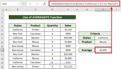
=AVERAGEIFS(C:C, A:A, "North", B:B, "Electronics")

Here, C:C is the range that contains the sales amounts you want to average, A:A is the range containing the regions, "North" is the criterion for the region, B:B is the range containing the product types, and "Electronics" is the criterion for the product type.

Breakdown of the Formula

• Average Range: C:C - This is the column that contains the sales amounts that you want to average.
• First Criteria Range: A:A - This is the column containing the regions.
• First Criteria: "North" - You're looking for sales in the North region.
• Second Criteria Range: B:B - This is the column containing the product types.
• Second Criteria: "Electronics" - You're interested in sales of Electronics products.

By applying this formula, you're telling Excel to average the sales amounts (found in column C) only for rows where the region is "North" (column A) and the product type is "Electronics" (column B).

Tips and Variations

• Dynamic Criteria: Instead of hardcoding your criteria like "North", you can reference cells that contain your criteria. For example, if you have a cell named E2 that contains the region you're interested in, you can use E2 in place of "North" in your formula.
• Multiple Criteria: One of the powerful features of AVERAGEIFS is the ability to apply multiple criteria. You can add as many criteria ranges and criteria as you need, separated by commas.
• Handling Errors: Be cautious with how you handle errors, especially if your data might include blank cells or errors that you don't want to average. You can use functions like IFERROR or IFBLANK to handle these situations gracefully.

Gallery of AVERAGEIFS Examples

AVERAGEIFS Examples Gallery

By mastering the AVERAGEIFS function, you can significantly enhance your data analysis capabilities in Excel, allowing you to more accurately and efficiently extract insights from your data.